
vaeffects.lib
Virtual Analog Effects (VAE) library. Its official prefix is ve.
This library provides virtual analog (VA) audio effects modeled after classic analog circuitry. It includes nonlinear filters and effects.
The virtual analog filter library is organized into 6 sections:
- Moog Filters
- Korg 35 Filters
- Oberheim Filters
- Sallen Key Filters
- Vicanek's Matched (Decramped) Second-Order Filters
- Effects
References
Moog Filters
(ve.)moog_vcf
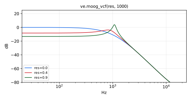
Moog "Voltage Controlled Filter" (VCF) in "analog" form. Moog VCF
implemented using the same logical block diagram as the classic
analog circuit. As such, it neglects the one-sample delay associated
with the feedback path around the four one-poles.
This extra delay alters the response, especially at high frequencies
(see reference [1] for details).
See moog_vcf_2b below for a more accurate implementation.
Usage
_ : moog_vcf(res,fr) : _
Where:
res: normalized amount of corner-resonance between 0 and 1 (0 is no resonance, 1 is maximum)fr: corner-resonance frequency in Hz. The filter is stable forfrbelow SR/6.28 atres<= 0.25, SR/6.88 at 0.5, SR/7.34 at 0.8 and SR/7.58 asresapproaches 1, so keepfrbelow about SR/7.6
Test
ve = library("vaeffects.lib");
os = library("oscillators.lib");
no = library("noises.lib");
ba = library("basics.lib");
ma = library("maths.lib");
moog_vcf_test = os.tosc(440) : ve.moog_vcf(0.5, 1000);
moog_vcf_slider_test = os.tosc(440)
  : ve.moog_vcf(
      hslider("moog_vcf:res", 0.5, 0, 1, 0.01),
      hslider("moog_vcf:freq", 1000, 50, 4000, 1)
    );
moog_vcf_modulated_test = no.noise : ve.moog_vcf(0.9, 50*pow(100, tri)) with { P = int(ma.SR/10); tri = 1 - abs(2*ba.period(P)/P - 1); };
moog_vcf_jump_test = no.noise : ve.moog_vcf(0.9, 50*pow(100, sq)) with { P = int(ma.SR/10); sq = ba.period(2*P) < P; };
moog_vcf_audio_modulated_test = 0.1*no.noise : ve.moog_vcf(0.9, max(20, 1000*(1 + 0.9*os.tosc(500))));
References
- https://ccrma.stanford.edu/~stilti/papers/moogvcf.pdf
- https://ccrma.stanford.edu/~jos/pasp/vegf.html
(ve.)moog_vcf_2b, (ve.)moog_vcf_2bn
Moog "Voltage Controlled Filter" (VCF) as two biquads. Implementation
of the ideal Moog VCF transfer function factored into second-order
sections. As a result, it is more accurate than moog_vcf above, but
its coefficient formulas are more complex when one or both parameters
are varied. Here, res is the fourth root of that in moog_vcf, so, as
the sampling rate approaches infinity, moog_vcf(res^4,fr) becomes equivalent
to moog_vcf_2b[n](res,fr) (when res and fr are constant).
moog_vcf_2b uses two direct-form biquads (tf2).
moog_vcf_2bn uses two protected normalized-ladder biquads (tf2np).
Usage
_ : moog_vcf_2b(res,fr) : _
_ : moog_vcf_2bn(res,fr) : _
Where:
res: normalized amount of corner-resonance between 0 and 1 (0 is min resonance, 1 is maximum)fr: corner-resonance frequency in Hz
Test
ve = library("vaeffects.lib");
os = library("oscillators.lib");
no = library("noises.lib");
ba = library("basics.lib");
ma = library("maths.lib");
moog_vcf_2b_test = os.tosc(330) : ve.moog_vcf_2b(0.4, 1200);
moog_vcf_2b_slider_test = os.tosc(330)
  : ve.moog_vcf_2b(
      hslider("moog_vcf_2b:res", 0.4, 0, 1, 0.01),
      hslider("moog_vcf_2b:freq", 1200, 50, 6000, 1)
    );
moog_vcf_2b_modulated_test = no.noise : ve.moog_vcf_2b(0.95, 20*pow(500, tri)) with { P = int(ma.SR/10); tri = 1 - abs(2*ba.period(P)/P - 1); };
moog_vcf_2b_jump_test = no.noise : ve.moog_vcf_2b(0.95, 20*pow(500, sq)) with { P = int(ma.SR/10); sq = ba.period(2*P) < P; };
moog_vcf_2bn_test = os.tosc(330) : ve.moog_vcf_2bn(0.4, 1200);
moog_vcf_2bn_slider_test = os.tosc(330)
  : ve.moog_vcf_2bn(
      hslider("moog_vcf_2bn:res", 0.4, 0, 1, 0.01),
      hslider("moog_vcf_2bn:freq", 1200, 50, 6000, 1)
    );
moog_vcf_2bn_modulated_test = no.noise : ve.moog_vcf_2bn(0.95, 20*pow(500, tri)) with { P = int(ma.SR/10); tri = 1 - abs(2*ba.period(P)/P - 1); };
moog_vcf_2bn_jump_test = no.noise : ve.moog_vcf_2bn(0.95, 20*pow(500, sq)) with { P = int(ma.SR/10); sq = ba.period(2*P) < P; };
moog_vcf_2b_audio_modulated_test = 0.1*no.noise : ve.moog_vcf_2b(0.95, max(20, 1000*(1 + 0.9*os.tosc(500))));
moog_vcf_2bn_audio_modulated_test = 0.1*no.noise : ve.moog_vcf_2bn(0.95, max(20, 1000*(1 + 0.9*os.tosc(500))));
(ve.)moogLadder
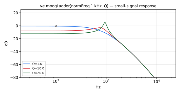
Virtual analog model of the 4th-order Moog Ladder (without any nonlinearities), which is arguably the most well-known ladder filter in analog synthesizers. Several 1st-order filters are cascaded in series. Feedback is then used, in part, to control the cut-off frequency and the resonance.
Usage
_ : moogLadder(normFreq,Q) : _
Where:
normFreq: normalized frequency (0-1)Q: quality factor between .707 (0 feedback coefficient) to 25 (feedback = 4, which is the self-oscillating threshold).
Test
ve = library("vaeffects.lib");
os = library("oscillators.lib");
no = library("noises.lib");
ba = library("basics.lib");
ma = library("maths.lib");
moogLadder_test = os.tosc(220) : ve.moogLadder(0.3, 4);
moogLadder_slider_test = os.tosc(220)
  : ve.moogLadder(
      hslider("moogLadder:normFreq", 0.3, 0, 1, 0.001),
      hslider("moogLadder:Q", 4, 0.7, 20, 0.1)
    );
moogLadder_modulated_test = no.noise : ve.moogLadder(0.8*tri, 20) with { P = int(ma.SR/10); tri = 1 - abs(2*ba.period(P)/P - 1); };
moogLadder_jump_test = no.noise : ve.moogLadder(0.8*sq, 20) with { P = int(ma.SR/10); sq = ba.period(2*P) < P; };
moogLadder_audio_modulated_test = 0.1*no.noise : ve.moogLadder(log10(max(20, 1000*(1 + 0.9*os.tosc(500)))/20)/3, 10);
References
- [Zavalishin 2012] (revision 2.1.2, February 2020)
- https://www.discodsp.net/VAFilterDesign_2.1.2.pdf
- Lorenzo Della Cioppa's correction to Pirkle's implementation: https://www.kvraudio.com/forum/viewtopic.php?f=33https://www.kvraudio.com/forum/viewtopic.php?f=33&t=571909t=571909
(ve.)lowpassLadder4
Topology-preserving transform implementation of a four-pole ladder lowpass. This is essentially the same filter as the moogLadder above except for the parameters, which will be expressed in Hz, for the cutoff, and as a raw feedback coefficient, for the resonance. Also, note that the parameter order has changed.
Usage
_ : lowpassLadder4(k, CF) : _
Where:
k: feedback coefficient between 0 and 4, which is the stability threshold.CF: the filter's cutoff in Hz.
Test
ve = library("vaeffects.lib");
os = library("oscillators.lib");
no = library("noises.lib");
ba = library("basics.lib");
ma = library("maths.lib");
lowpassLadder4_test = os.tosc(110) : ve.lowpassLadder4(2.0, 800);
lowpassLadder4_slider_test = os.tosc(110)
  : ve.lowpassLadder4(
      hslider("lowpassLadder4:k", 2.0, 0, 4, 0.1),
      hslider("lowpassLadder4:freq", 800, 50, 5000, 1)
    );
lowpassLadder4_modulated_test = no.noise : ve.lowpassLadder4(3.9, 20*pow(250, tri)) with { P = int(ma.SR/10); tri = 1 - abs(2*ba.period(P)/P - 1); };
lowpassLadder4_jump_test = no.noise : ve.lowpassLadder4(3.9, 20*pow(250, sq)) with { P = int(ma.SR/10); sq = ba.period(2*P) < P; };
lowpassLadder4_audio_modulated_test = 0.1*no.noise : ve.lowpassLadder4(3.9, max(20, 1000*(1 + 0.9*os.tosc(500))));
Notes:
If you want to express the feedback coefficient as the resonance peak, you can use the formula:
k = 4.0 - 1.0 / Q;
where Q, between .25 and infinity, corresponds to the peak of the filter at cutoff. I.e., if you feed the filter with a sine whose frequency is the same as the cutoff, the output peak corresponds exactly to that set via the Q-param.
References
- [Zavalishin 2012] (revision 2.1.2, February 2020)
- https://www.discodsp.net/VAFilterDesign_2.1.2.pdf
(ve.)moogHalfLadder
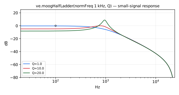
Virtual analog model of the 2nd-order Moog Half Ladder (simplified version of
(ve.)moogLadder). Several 1st-order filters are cascaded in series.
Feedback is then used, in part, to control the cut-off frequency and the
resonance.
This filter was implemented in Faust by Eric Tarr during the 2019 Embedded DSP With Faust Workshop.
Usage
_ : moogHalfLadder(normFreq,Q) : _
Where:
normFreq: normalized frequency (0-1)Q: q
Test
ve = library("vaeffects.lib");
os = library("oscillators.lib");
no = library("noises.lib");
ba = library("basics.lib");
ma = library("maths.lib");
moogHalfLadder_test = os.tosc(220) : ve.moogHalfLadder(0.3, 4);
moogHalfLadder_slider_test = os.tosc(220)
  : ve.moogHalfLadder(
      hslider("moogHalfLadder:normFreq", 0.3, 0, 1, 0.001),
      hslider("moogHalfLadder:Q", 4, 0.7, 20, 0.1)
    );
moogHalfLadder_modulated_test = no.noise : ve.moogHalfLadder(0.8*tri, 20) with { P = int(ma.SR/10); tri = 1 - abs(2*ba.period(P)/P - 1); };
moogHalfLadder_jump_test = no.noise : ve.moogHalfLadder(0.8*sq, 20) with { P = int(ma.SR/10); sq = ba.period(2*P) < P; };
moogHalfLadder_audio_modulated_test = 0.1*no.noise : ve.moogHalfLadder(log10(max(20, 1000*(1 + 0.9*os.tosc(500)))/20)/3, 10);
References
- https://www.willpirkle.com/app-notes/virtual-analog-moog-half-ladder-filter
- http://www.willpirkle.com/Downloads/AN-8MoogHalfLadderFilter.pdf
(ve.)diodeLadder
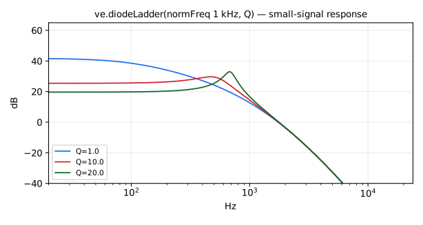
4th order virtual analog diode ladder filter. In addition to the individual
states used within each independent 1st-order filter, there are also additional
feedback paths found in the block diagram. These feedback paths are labeled
as connecting states. Rather than separately storing these connecting states
in the Faust implementation, they are simply implicitly calculated by
tracing back to the other states (s1,s2,s3,s4) each recursive step.
This filter was implemented in Faust by Eric Tarr during the 2019 Embedded DSP With Faust Workshop.
Usage
_ : diodeLadder(normFreq,Q) : _
Where:
normFreq: normalized frequency (0-1)Q: q
Test
ve = library("vaeffects.lib");
os = library("oscillators.lib");
no = library("noises.lib");
ba = library("basics.lib");
ma = library("maths.lib");
diodeLadder_test = os.tosc(220) : ve.diodeLadder(0.4, 4);
diodeLadder_slider_test = os.tosc(220)
  : ve.diodeLadder(
      hslider("diodeLadder:normFreq", 0.4, 0, 1, 0.001),
      hslider("diodeLadder:Q", 4, 0.7, 20, 0.1)
    );
diodeLadder_modulated_test = no.noise : ve.diodeLadder(0.8*tri, 20) with { P = int(ma.SR/10); tri = 1 - abs(2*ba.period(P)/P - 1); };
diodeLadder_jump_test = no.noise : ve.diodeLadder(0.8*sq, 20) with { P = int(ma.SR/10); sq = ba.period(2*P) < P; };
diodeLadder_audio_modulated_test = 0.1*no.noise : ve.diodeLadder(log10(max(20, 1000*(1 + 0.9*os.tosc(500)))/20)/3, 10);
References
- https://www.willpirkle.com/virtual-analog-diode-ladder-filter/
- http://www.willpirkle.com/Downloads/AN-6DiodeLadderFilter.pdf
Korg 35 Filters
The following filters are virtual analog models of the Korg 35 low-pass filter and high-pass filter found in the MS-10 and MS-20 synthesizers. The virtual analog models for the LPF and HPF are different, making these filters more interesting than simply tapping different states of the same circuit.
These filters were implemented in Faust by Eric Tarr during the 2019 Embedded DSP With Faust Workshop.
Filter history:
(ve.)korg35LPF
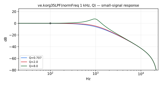
Virtual analog models of the Korg 35 low-pass filter found in the MS-10 and MS-20 synthesizers.
Usage
_ : korg35LPF(normFreq,Q) : _
Where:
normFreq: normalized frequency (0-1)Q: q
Test
ve = library("vaeffects.lib");
os = library("oscillators.lib");
no = library("noises.lib");
ba = library("basics.lib");
ma = library("maths.lib");
korg35LPF_test = os.tosc(220) : ve.korg35LPF(0.35, 3.5);
korg35LPF_slider_test = os.tosc(220)
  : ve.korg35LPF(
      hslider("korg35LPF:normFreq", 0.35, 0, 1, 0.001),
      hslider("korg35LPF:Q", 3.5, 0.7, 10, 0.1)
    );
korg35LPF_modulated_test = no.noise : ve.korg35LPF(0.8*tri, 9.5) with { P = int(ma.SR/10); tri = 1 - abs(2*ba.period(P)/P - 1); };
korg35LPF_jump_test = no.noise : ve.korg35LPF(0.8*sq, 9.5) with { P = int(ma.SR/10); sq = ba.period(2*P) < P; };
korg35LPF_audio_modulated_test = 0.1*no.noise : ve.korg35LPF(log10(max(20, 1000*(1 + 0.9*os.tosc(500)))/20)/3, 9.5);
(ve.)korg35HPF
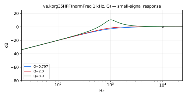
Virtual analog models of the Korg 35 high-pass filter found in the MS-10 and MS-20 synthesizers.
Usage
_ : korg35HPF(normFreq,Q) : _
Where:
normFreq: normalized frequency (0-1)Q: q
Test
ve = library("vaeffects.lib");
os = library("oscillators.lib");
no = library("noises.lib");
ba = library("basics.lib");
ma = library("maths.lib");
korg35HPF_test = os.tosc(330) : ve.korg35HPF(0.4, 3.5);
korg35HPF_slider_test = os.tosc(330)
  : ve.korg35HPF(
      hslider("korg35HPF:normFreq", 0.4, 0, 1, 0.001),
      hslider("korg35HPF:Q", 3.5, 0.7, 10, 0.1)
    );
korg35HPF_modulated_test = no.noise : ve.korg35HPF(0.8*tri, 9.5) with { P = int(ma.SR/10); tri = 1 - abs(2*ba.period(P)/P - 1); };
korg35HPF_jump_test = no.noise : ve.korg35HPF(0.8*sq, 9.5) with { P = int(ma.SR/10); sq = ba.period(2*P) < P; };
korg35HPF_audio_modulated_test = 0.1*no.noise : ve.korg35HPF(log10(max(20, 1000*(1 + 0.9*os.tosc(500)))/20)/3, 9.5);
Oberheim Filters
The following filter (4 types) is an implementation of the virtual analog model described in Section 7.2 of the Will Pirkle book, "Designing Software Synthesizer Plug-ins in C++". It is based on the block diagram in Figure 7.5.
The Oberheim filter is a state-variable filter with soft-clipping distortion within the circuit.
In many VA filters, distortion is accomplished using the "tanh" function.
For this Faust implementation, that distortion function was replaced with
the (ef.)cubicnl function.
(ve.)oberheim
Generic multi-outputs Oberheim filter that produces the BSF, BPF, HPF and LPF outputs (see description above).
Usage
_ : oberheim(normFreq,Q) : _,_,_,_
Where:
normFreq: normalized frequency (0-1)Q: q
Test
ve = library("vaeffects.lib");
os = library("oscillators.lib");
no = library("noises.lib");
ba = library("basics.lib");
ma = library("maths.lib");
oberheim_test = os.tosc(220) : ve.oberheim(0.4, 1.5);
oberheim_slider_test = os.tosc(220)
  : ve.oberheim(
      hslider("oberheim:normFreq", 0.4, 0, 1, 0.001),
      hslider("oberheim:Q", 1.5, 0.5, 10, 0.1)
    );
oberheim_modulated_test = no.noise : ve.oberheim(0.8*tri, 10) with { P = int(ma.SR/10); tri = 1 - abs(2*ba.period(P)/P - 1); };
oberheim_jump_test = no.noise : ve.oberheim(0.8*sq, 10) with { P = int(ma.SR/10); sq = ba.period(2*P) < P; };
oberheim_audio_modulated_test = 0.1*no.noise : ve.oberheim(log10(max(20, 1000*(1 + 0.9*os.tosc(500)))/20)/3, 10);
(ve.)oberheimBSF
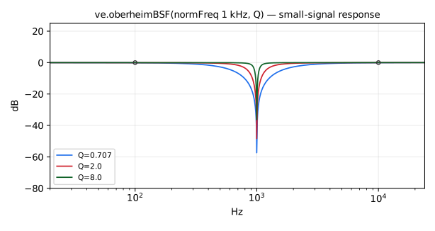
Band-Stop Oberheim filter (see description above). Specialize the generic implementation: keep the first BSF output, the compiler will only generate the needed code.
Usage
_ : oberheimBSF(normFreq,Q) : _
Where:
normFreq: normalized frequency (0-1)Q: q
Test
ve = library("vaeffects.lib");
os = library("oscillators.lib");
oberheimBSF_test = os.tosc(220) : ve.oberheimBSF(0.4, 1.5);
oberheimBSF_slider_test = os.tosc(220)
  : ve.oberheimBSF(
      hslider("oberheimBSF:normFreq", 0.4, 0, 1, 0.001),
      hslider("oberheimBSF:Q", 1.5, 0.5, 10, 0.1)
    );
(ve.)oberheimBPF
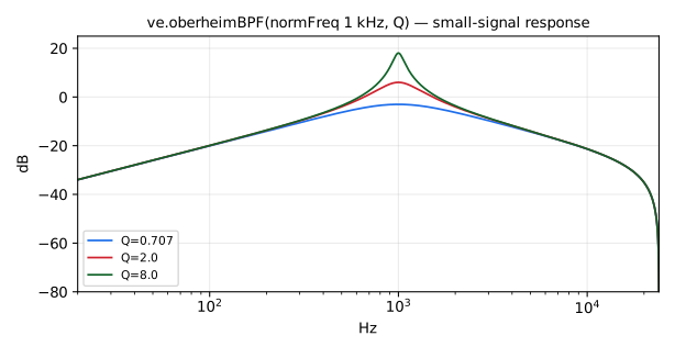
Band-Pass Oberheim filter (see description above). Specialize the generic implementation: keep the second BPF output, the compiler will only generate the needed code.
Usage
_ : oberheimBPF(normFreq,Q) : _
Where:
normFreq: normalized frequency (0-1)Q: q
Test
ve = library("vaeffects.lib");
os = library("oscillators.lib");
oberheimBPF_test = os.tosc(220) : ve.oberheimBPF(0.4, 1.5);
oberheimBPF_slider_test = os.tosc(220)
  : ve.oberheimBPF(
      hslider("oberheimBPF:normFreq", 0.4, 0, 1, 0.001),
      hslider("oberheimBPF:Q", 1.5, 0.5, 10, 0.1)
    );
(ve.)oberheimHPF
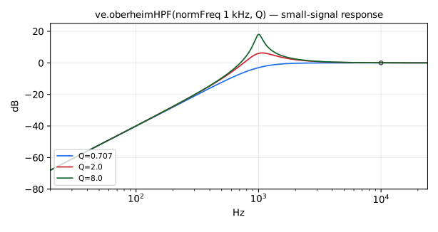
High-Pass Oberheim filter (see description above). Specialize the generic implementation: keep the third HPF output, the compiler will only generate the needed code.
Usage
_ : oberheimHPF(normFreq,Q) : _
Where:
normFreq: normalized frequency (0-1)Q: q
Test
ve = library("vaeffects.lib");
os = library("oscillators.lib");
oberheimHPF_test = os.tosc(220) : ve.oberheimHPF(0.4, 1.5);
oberheimHPF_slider_test = os.tosc(220)
  : ve.oberheimHPF(
      hslider("oberheimHPF:normFreq", 0.4, 0, 1, 0.001),
      hslider("oberheimHPF:Q", 1.5, 0.5, 10, 0.1)
    );
(ve.)oberheimLPF
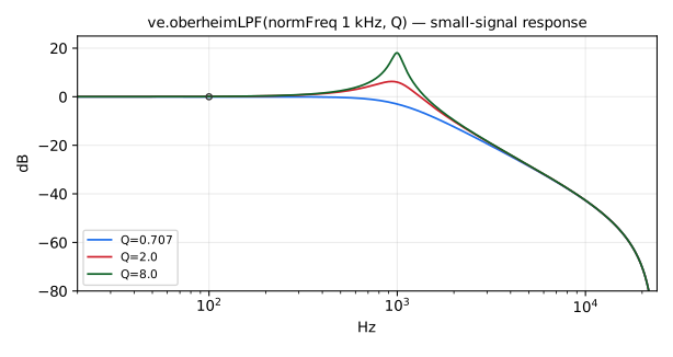
Low-Pass Oberheim filter (see description above). Specialize the generic implementation: keep the fourth LPF output, the compiler will only generate the needed code.
Usage
_ : oberheimLPF(normFreq,Q) : _
Where:
normFreq: normalized frequency (0-1)Q: q
Test
ve = library("vaeffects.lib");
os = library("oscillators.lib");
oberheimLPF_test = os.tosc(220) : ve.oberheimLPF(0.4, 1.5);
oberheimLPF_slider_test = os.tosc(220)
  : ve.oberheimLPF(
      hslider("oberheimLPF:normFreq", 0.4, 0, 1, 0.001),
      hslider("oberheimLPF:Q", 1.5, 0.5, 10, 0.1)
    );
Sallen Key Filters
The following filters were implemented based on VA models of synthesizer filters.
The modeling approach is based on a Topology Preserving Transform (TPT) to resolve the delay-free feedback loop in the corresponding analog filters.
The primary processing block used to build other filters (Moog, Korg, etc.) is based on a 1st-order Sallen-Key filter.
The filters included in this script are 1st-order LPF/HPF and 2nd-order state-variable filters capable of LPF, HPF, and BPF.
Resources:
- Vadim Zavalishin (2018) "The Art of VA Filter Design", v2.1.0
- https://www.discodsp.net/VAFilterDesign_2.1.0.pdf
- Will Pirkle (2014) "Resolving Delay-Free Loops in Recursive Filters Using the Modified Härmä Method", AES 137 http://www.aes.org/e-lib/browse.cfm?elib=17517
- Description and diagrams of 1st- and 2nd-order TPT filters:
- https://www.willpirkle.com/706-2/
(ve.)sallenKeyOnePole
Sallen-Key generic One Pole filter that produces the LPF and HPF outputs (see description above).
For the Faust implementation of this filter, recursion (letrec) is used
for storing filter "states". The output (e.g. y) is calculated by using
the input signal and the previous states of the filter.
During the current recursive step, the states of the filter (e.g. s) for
the next step are also calculated.
Admittedly, this is not an efficient way to implement a filter because it requires independently calculating the output and each state during each recursive step. However, it works as a way to store and use "states" within the constraints of Faust.
The simplest example is the 1st-order LPF (shown on the cover of Zavalishin 2018 and Fig 4.3 of https://www.willpirkle.com/706-2/).
Here, the input signal is split in parallel for the calculation of the output signal, y,
and the state s. The value of the state is only used for feedback to the next
step of recursion. It is blocked (!) from also being routed to the output.
A trick used for calculating the state s is to observe that the input to
the delay block is the sum of two signal: what appears to be a feedforward
path and a feedback path. In reality, the signals being summed are identical
(signal*2) plus the value of the current state.
Usage
_ : sallenKeyOnePole(normFreq) : _,_
Where:
normFreq: normalized frequency (0-1)
Test
ve = library("vaeffects.lib");
os = library("oscillators.lib");
no = library("noises.lib");
ba = library("basics.lib");
ma = library("maths.lib");
sallenKeyOnePole_test = os.tosc(440) : ve.sallenKeyOnePole(0.25);
sallenKeyOnePole_slider_test = os.tosc(440)
  : ve.sallenKeyOnePole(
      hslider("sallenKeyOnePole:normFreq", 0.25, 0, 1, 0.001)
    );
sallenKeyOnePole_modulated_test = no.noise : ve.sallenKeyOnePole(0.8*tri) with { P = int(ma.SR/10); tri = 1 - abs(2*ba.period(P)/P - 1); };
sallenKeyOnePole_jump_test = no.noise : ve.sallenKeyOnePole(0.8*sq) with { P = int(ma.SR/10); sq = ba.period(2*P) < P; };
(ve.)sallenKeyOnePoleLPF
Sallen-Key One Pole lowpass filter (see description above). Specialize the generic implementation: keep the first LPF output, the compiler will only generate the needed code.
Usage
_ : sallenKeyOnePoleLPF(normFreq) : _
Where:
normFreq: normalized frequency (0-1)
Test
ve = library("vaeffects.lib");
os = library("oscillators.lib");
sallenKeyOnePoleLPF_test = os.tosc(440) : ve.sallenKeyOnePoleLPF(0.25);
sallenKeyOnePoleLPF_slider_test = os.tosc(440)
  : ve.sallenKeyOnePoleLPF(
      hslider("sallenKeyOnePoleLPF:normFreq", 0.25, 0, 1, 0.001)
    );
(ve.)sallenKeyOnePoleHPF
Sallen-Key One Pole Highpass filter (see description above). The dry input signal is routed in parallel to the output. The LPF'd signal is subtracted from the input so that the HPF remains. Specialize the generic implementation: keep the second HPF output, the compiler will only generate the needed code.
Usage
_ : sallenKeyOnePoleHPF(normFreq) : _
Where:
normFreq: normalized frequency (0-1)
Test
ve = library("vaeffects.lib");
os = library("oscillators.lib");
sallenKeyOnePoleHPF_test = os.tosc(440) : ve.sallenKeyOnePoleHPF(0.25);
sallenKeyOnePoleHPF_slider_test = os.tosc(440)
  : ve.sallenKeyOnePoleHPF(
      hslider("sallenKeyOnePoleHPF:normFreq", 0.25, 0, 1, 0.001)
    );
(ve.)sallenKey2ndOrder
Sallen-Key generic 2nd order filter that produces the LPF, BPF and HPF outputs.
This is a 2nd-order Sallen-Key state-variable filter. The idea is that by "tapping" into different points in the circuit, different filters (LPF,BPF,HPF) can be achieved. See Figure 4.6 of https://www.willpirkle.com/706-2/
This is also a good example of the next step for generalizing the Faust
programming approach used for all these VA filters. In this case, there are
three things to calculate each recursive step (y,s1,s2). For each thing, the
circuit is only calculated up to that point.
Comparing the LPF to BPF, the output signal (y) is calculated similarly.
Except, the output of the BPF stops earlier in the circuit. Similarly, the
states (s1 and s2) only differ in that s2 includes a couple more terms
beyond what is used for s1.
Usage
_ : sallenKey2ndOrder(normFreq,Q) : _,_,_
Where:
normFreq: normalized frequency (0-1)Q: quality factor controlling the sharpness/resonance of the filter around the center frequency (CF). For bandpass filters, higher Q increases the gain at the center frequency. Must be in the range[ma.EPSILON, ma.MAX]
Test
ve = library("vaeffects.lib");
os = library("oscillators.lib");
no = library("noises.lib");
ba = library("basics.lib");
ma = library("maths.lib");
sallenKey2ndOrder_test = os.tosc(330) : ve.sallenKey2ndOrder(0.3, 1.0);
sallenKey2ndOrder_slider_test = os.tosc(330)
  : ve.sallenKey2ndOrder(
      hslider("sallenKey2ndOrder:normFreq", 0.3, 0, 1, 0.001),
      hslider("sallenKey2ndOrder:Q", 1.0, 0.1, 10, 0.1)
    );
sallenKey2ndOrder_modulated_test = no.noise : ve.sallenKey2ndOrder(0.8*tri, 10) with { P = int(ma.SR/10); tri = 1 - abs(2*ba.period(P)/P - 1); };
sallenKey2ndOrder_jump_test = no.noise : ve.sallenKey2ndOrder(0.8*sq, 10) with { P = int(ma.SR/10); sq = ba.period(2*P) < P; };
sallenKey2ndOrder_audio_modulated_test = 0.1*no.noise : ve.sallenKey2ndOrder(log10(max(20, 1000*(1 + 0.9*os.tosc(500)))/20)/3, 10);
(ve.)sallenKey2ndOrderLPF
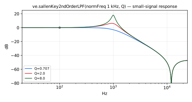
Sallen-Key 2nd order lowpass filter (see description above). Specialize the generic implementation: keep the first LPF output, the compiler will only generate the needed code.
Usage
_ : sallenKey2ndOrderLPF(normFreq,Q) : _
Where:
normFreq: normalized frequency (0-1)Q: quality factor controlling the sharpness/resonance of the filter around the center frequency (CF). For bandpass filters, higher Q increases the gain at the center frequency. Must be in the range[ma.EPSILON, ma.MAX]
Test
ve = library("vaeffects.lib");
os = library("oscillators.lib");
sallenKey2ndOrderLPF_test = os.tosc(330) : ve.sallenKey2ndOrderLPF(0.3, 0.8);
sallenKey2ndOrderLPF_slider_test = os.tosc(330)
  : ve.sallenKey2ndOrderLPF(
      hslider("sallenKey2ndOrderLPF:normFreq", 0.3, 0, 1, 0.001),
      hslider("sallenKey2ndOrderLPF:Q", 0.8, 0.1, 10, 0.1)
    );
(ve.)sallenKey2ndOrderBPF
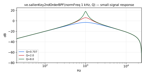
Sallen-Key 2nd order bandpass filter (see description above). Specialize the generic implementation: keep the second BPF output, the compiler will only generate the needed code.
Usage
_ : sallenKey2ndOrderBPF(normFreq,Q) : _
Where:
normFreq: normalized frequency (0-1)Q: quality factor controlling the sharpness/resonance of the filter around the center frequency (CF). For bandpass filters, higher Q increases the gain at the center frequency. Must be in the range[ma.EPSILON, ma.MAX]
Test
ve = library("vaeffects.lib");
os = library("oscillators.lib");
sallenKey2ndOrderBPF_test = os.tosc(330) : ve.sallenKey2ndOrderBPF(0.3, 1.5);
sallenKey2ndOrderBPF_slider_test = os.tosc(330)
  : ve.sallenKey2ndOrderBPF(
      hslider("sallenKey2ndOrderBPF:normFreq", 0.3, 0, 1, 0.001),
      hslider("sallenKey2ndOrderBPF:Q", 1.5, 0.1, 10, 0.1)
    );
(ve.)sallenKey2ndOrderHPF
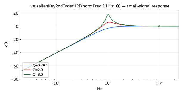
Sallen-Key 2nd order highpass filter (see description above). Specialize the generic implementation: keep the third HPF output, the compiler will only generate the needed code.
Usage
_ : sallenKey2ndOrderHPF(normFreq,Q) : _
Where:
normFreq: normalized frequency (0-1)Q: quality factor controlling the sharpness/resonance of the filter around the center frequency (CF). For bandpass filters, higher Q increases the gain at the center frequency. Must be in the range[ma.EPSILON, ma.MAX]
Test
ve = library("vaeffects.lib");
os = library("oscillators.lib");
sallenKey2ndOrderHPF_test = os.tosc(330) : ve.sallenKey2ndOrderHPF(0.3, 0.8);
sallenKey2ndOrderHPF_slider_test = os.tosc(330)
  : ve.sallenKey2ndOrderHPF(
      hslider("sallenKey2ndOrderHPF:normFreq", 0.3, 0, 1, 0.001),
      hslider("sallenKey2ndOrderHPF:Q", 0.8, 0.1, 10, 0.1)
    );
Vicanek's Matched (Decramped) Second-Order Filters
Vicanek's Matched (Decramped) Second-Order Filters.
This collection implements high-quality second-order filters based on the work of Vicanek, offering improved frequency accuracy and dynamic response over traditional biquads—especially near Nyquist.
Standard digital filter designs (like bilinear-transformed biquads) suffer from frequency warping, which distorts the placement of poles and zeros. Vicanek's method, detailed in his paper "Matched Second Order Digital Filters", proposes a set of matched filter formulas that eliminate such warping, preserving the intended analog-like behavior and frequency response.
The filters provided here include:
biquad— generic difference equation implementationlowpass2Matched— second-order lowpass with resonancehighpass2Matched— second-order highpass with resonancebandpass2Matched— second-order bandpass with resonancepeaking2Matched— second-order peaking EQlowshelf2Matched– second-order Butterworth lowshelfhighshelf2Matched– second-order Butterworth highshelf
Each filter relies on carefully derived coefficient formulas that guarantee accurate placement of the frequency response peak and preserve Q and gain behavior.
Their coefficients are computed without cancellation and their recurrence
runs on small increments, so that they are accurate in single precision too,
at every sample rate: a low CF or a high Q stays within about 1e-5 of the
double-precision output (1e-4 for bandpass2Matched).
References
- Vicanek, M. (2016) Matched Second Order Digital Filters
- https://www.vicanek.de/articles/BiquadFits.pdf
(ve.)biquad
Basic biquad section implementing the difference equation:
y[n] = b0 * x[n] + b1 * x[n-1] + b2 * x[n-2] - a1 * y[n-1] - a2 * y[n-2]
Usage:
_ : biquad(b0, b1, b2, a1, a2) : _
Where:
b0: feedforward coefficient forx[n]b1: feedforward coefficient forx[n-1]b2: feedforward coefficient forx[n-2]a1: feedback coefficient fory[n-1]a2: feedback coefficient fory[n-2]
Test
ve = library("vaeffects.lib");
os = library("oscillators.lib");
biquad_test = os.tosc(440)
  : ve.biquad(0.5, 0.3, 0.2, -0.3, 0.2);
(ve.)lowpass2Matched
Vicanek's decramped second-order resonant lowpass filter.
Accurate in single precision too: its coefficients are computed without
cancellation and its recurrence runs on small increments, so that a low
CF or a high Q at a high sample rate stays within about 1e-5 of the
double-precision output.
Usage:
_ : lowpass2Matched(CF, Q) : _
Where:
CF: cutoff frequency in HzQ: resonance linear amplitude
Test
ve = library("vaeffects.lib");
os = library("oscillators.lib");
no = library("noises.lib");
ba = library("basics.lib");
ma = library("maths.lib");
lowpass2Matched_test = os.tosc(440) : ve.lowpass2Matched(1000, 0.707);
lowpass2Matched_slider_test = os.tosc(440)
  : ve.lowpass2Matched(
      hslider("lowpass2Matched:CF", 1000, 50, 5000, 1),
      hslider("lowpass2Matched:Q", 0.707, 0.1, 5, 0.01)
    );
lowpass2Matched_modulated_test = no.noise : ve.lowpass2Matched(20*pow(250, tri), 5) with { P = int(ma.SR/10); tri = 1 - abs(2*ba.period(P)/P - 1); };
lowpass2Matched_low_test = no.noise : ve.lowpass2Matched(50, 10);
(ve.)highpass2Matched
Vicanek's decramped second-order resonant highpass filter.
Accurate in single precision too: its coefficients are computed without
cancellation and its recurrence runs on small increments, so that a low
CF or a high Q at a high sample rate stays within about 1e-5 of the
double-precision output.
Usage:
_ : highpass2Matched(CF, Q) : _
Where:
CF: cutoff frequency in HzQ: resonance linear amplitude
Test
ve = library("vaeffects.lib");
os = library("oscillators.lib");
no = library("noises.lib");
ba = library("basics.lib");
ma = library("maths.lib");
highpass2Matched_test = os.tosc(440) : ve.highpass2Matched(500, 0.707);
highpass2Matched_slider_test = os.tosc(440)
  : ve.highpass2Matched(
      hslider("highpass2Matched:CF", 500, 50, 5000, 1),
      hslider("highpass2Matched:Q", 0.707, 0.1, 5, 0.01)
    );
highpass2Matched_modulated_test = no.noise : ve.highpass2Matched(20*pow(250, tri), 5) with { P = int(ma.SR/10); tri = 1 - abs(2*ba.period(P)/P - 1); };
highpass2Matched_low_test = no.noise : ve.highpass2Matched(50, 10);
(ve.)bandpass2Matched
Vicanek's decramped second-order resonant bandpass filter.
Accurate in single precision too: its coefficients are computed without
cancellation and its recurrence runs on small increments, so that a low
CF or a high Q at a high sample rate stays within about 1e-4 of the
double-precision output.
Usage:
_ : bandpass2Matched(CF, Q) : _
Where:
CF: cutoff frequency in HzQ: peak width
Test
ve = library("vaeffects.lib");
os = library("oscillators.lib");
no = library("noises.lib");
ba = library("basics.lib");
ma = library("maths.lib");
bandpass2Matched_test = os.tosc(440) : ve.bandpass2Matched(1200, 2.0);
bandpass2Matched_slider_test = os.tosc(440)
  : ve.bandpass2Matched(
      hslider("bandpass2Matched:CF", 1200, 50, 5000, 1),
      hslider("bandpass2Matched:Q", 2.0, 0.1, 10, 0.01)
    );
bandpass2Matched_modulated_test = no.noise : ve.bandpass2Matched(20*pow(250, tri), 5) with { P = int(ma.SR/10); tri = 1 - abs(2*ba.period(P)/P - 1); };
bandpass2Matched_low_test = no.noise : ve.bandpass2Matched(50, 10);
(ve.)peaking2Matched
Vicanek's decramped second-order peaking equalizer.
Accurate in single precision too: its coefficients are computed without
cancellation and its recurrence runs on small increments, so that a low
CF or a high Q at a high sample rate stays within about 1e-5 of the
double-precision output.
Usage:
_ : peaking2Matched(G, CF, Q) : _
Where:
G: peak linear amplitudeCF: cutoff frequency in HzQ: peak width
Test
ve = library("vaeffects.lib");
os = library("oscillators.lib");
no = library("noises.lib");
ba = library("basics.lib");
ma = library("maths.lib");
peaking2Matched_test = os.tosc(440) : ve.peaking2Matched(1.5, 1000, 2.0);
peaking2Matched_slider_test = os.tosc(440)
  : ve.peaking2Matched(
      hslider("peaking2Matched:G", 1.5, 0.1, 4, 0.01),
      hslider("peaking2Matched:CF", 1000, 50, 5000, 1),
      hslider("peaking2Matched:Q", 2.0, 0.1, 10, 0.01)
    );
peaking2Matched_modulated_test = no.noise : ve.peaking2Matched(2, 20*pow(250, tri), 5) with { P = int(ma.SR/10); tri = 1 - abs(2*ba.period(P)/P - 1); };
peaking2Matched_low_test = no.noise : ve.peaking2Matched(4, 50, 10);
(ve.)lowshelf2Matched
Vicanek's decramped second-order Butterworth lowshelf filter.
Accurate in single precision too: its coefficients are computed without
cancellation and its recurrence runs on small increments, so that a low
CF at a high sample rate stays within about 1e-5 of the double-precision
output. G = 1 gives the identity.
Usage:
_ : lowshelf2Matched(G, CF) : _
Where:
G: shelf linear amplitudeCF: cutoff frequency in Hz
Test
ve = library("vaeffects.lib");
os = library("oscillators.lib");
no = library("noises.lib");
ba = library("basics.lib");
ma = library("maths.lib");
lowshelf2Matched_test = os.tosc(330) : ve.lowshelf2Matched(1.5, 500);
lowshelf2Matched_slider_test = os.tosc(330)
  : ve.lowshelf2Matched(
      hslider("lowshelf2Matched:G", 1.5, 0.5, 4, 0.01),
      hslider("lowshelf2Matched:CF", 500, 50, 5000, 1)
    );
lowshelf2Matched_modulated_test = no.noise : ve.lowshelf2Matched(0.25*pow(16, tri), 1000) with { P = int(ma.SR/10); tri = 1 - abs(2*ba.period(P)/P - 1); };
lowshelf2Matched_low_test = no.noise : ve.lowshelf2Matched(4, 20);
lowshelf2Matched_unity_test = no.noise : ve.lowshelf2Matched(1, 500);
(ve.)highshelf2Matched
Vicanek's decramped second-order Butterworth highshelf filter.
Accurate in single precision too: its coefficients are computed without
cancellation and its recurrence runs on small increments, so that a low
CF at a high sample rate stays within about 1e-5 of the double-precision
output. G = 1 gives the identity.
Usage:
_ : highshelf2Matched(G, CF) : _
Where:
G: shelf linear amplitudeCF: cutoff frequency in Hz
Test
ve = library("vaeffects.lib");
os = library("oscillators.lib");
no = library("noises.lib");
ba = library("basics.lib");
ma = library("maths.lib");
highshelf2Matched_test = os.tosc(330) : ve.highshelf2Matched(1.5, 1500);
highshelf2Matched_slider_test = os.tosc(330)
  : ve.highshelf2Matched(
      hslider("highshelf2Matched:G", 1.5, 0.5, 4, 0.01),
      hslider("highshelf2Matched:CF", 1500, 50, 10000, 1)
    );
highshelf2Matched_modulated_test = no.noise : ve.highshelf2Matched(0.25*pow(16, tri), 1000) with { P = int(ma.SR/10); tri = 1 - abs(2*ba.period(P)/P - 1); };
highshelf2Matched_low_test = no.noise : ve.highshelf2Matched(0.25, 20);
highshelf2Matched_unity_test = no.noise : ve.highshelf2Matched(1, 500);
Effects
(ve.)wah4
Wah effect, 4th order.
wah4 is a standard Faust function.
Usage
_ : wah4(fr) : _
Where:
fr: resonance frequency in Hz, between 0 and SR/7.34 (about 6 kHz at 44.1 kHz). Above, or below 0, the filter is unstable.
Test
ve = library("vaeffects.lib");
os = library("oscillators.lib");
no = library("noises.lib");
ba = library("basics.lib");
ma = library("maths.lib");
wah4_test = os.tosc(220) : ve.wah4(800);
wah4_slider_test = os.tosc(220)
  : ve.wah4(
      hslider("wah4:freq", 800, 200, 2000, 1)
    );
wah4_modulated_test = no.noise : ve.wah4(200*pow(10, tri)) with { P = int(ma.SR/10); tri = 1 - abs(2*ba.period(P)/P - 1); };
References
(ve.)autowah
Auto-wah effect: crybaby with its wah parameter driven by the
input's amplitude envelope (an.amp_follower). Input peaks above 1
hold the pedal fully forward (crybaby clamps wah to [0,1]).
autowah is a standard Faust function.
Usage
_ : autowah(level) : _
Where:
level: amount of effect desired (0 to 1).
Test
ve = library("vaeffects.lib");
os = library("oscillators.lib");
no = library("noises.lib");
autowah_test = os.tosc(220) : ve.autowah(0.7);
autowah_slider_test = os.tosc(220)
  : ve.autowah(
      hslider("autowah:level", 0.7, 0, 1, 0.01)
    );
autowah_hot_test = 4*no.noise : ve.autowah(1);
(ve.)crybaby
Digitized CryBaby wah pedal.
crybaby is a standard Faust function.
Usage
_ : crybaby(wah) : _
Where:
wah: "pedal angle" from 0 to 1. Values outside are clamped to this range: without the clamp, the poles leave the unit circle above about 2.08 at 44.1 kHz (2.58 at 192 kHz).
Test
ve = library("vaeffects.lib");
os = library("oscillators.lib");
no = library("noises.lib");
ba = library("basics.lib");
ma = library("maths.lib");
crybaby_test = os.tosc(220) : ve.crybaby(0.3);
crybaby_slider_test = os.tosc(220)
  : ve.crybaby(
      hslider("crybaby:wah", 0.3, 0, 1, 0.01)
    );
crybaby_modulated_test = no.noise : ve.crybaby(tri) with { P = int(ma.SR/10); tri = 1 - abs(2*ba.period(P)/P - 1); };
crybaby_jump_test = no.noise : ve.crybaby(sq) with { P = int(ma.SR/10); sq = ba.period(2*P) < P; };
crybaby_noise_test = no.noise : ve.crybaby(0);
crybaby_clamp_test = no.noise <: ve.crybaby(-1), ve.crybaby(3);
References
(ve.)vocoder
A very simple vocoder where the spectrum of the modulation signal
is analyzed using a filter bank.
vocoder is a standard Faust function.
The two signals can also be given as inputs, by partial application
(second form below, as in the Test section).
Usage
vocoder(nBands,att,rel,BWRatio,source,excitation) : _
source, excitation : vocoder(nBands,att,rel,BWRatio) : _
Where:
nBands: Number of vocoder bandsatt: Attack time in secondsrel: Release time in secondsBWRatio: Coefficient to adjust the bandwidth of each band (0.1 - 2)source: Modulation signalexcitation: Excitation/Carrier signal
Test
ve = library("vaeffects.lib");
no = library("noises.lib");
os = library("oscillators.lib");
vocoder_test = (no.noise, os.tosc(220)) : ve.vocoder(8, 0.01, 0.1, 1.0);
vocoder_slider_test = (no.noise, os.tosc(220))
  : ve.vocoder(
      8,
      hslider("vocoder:att", 0.01, 0.001, 0.1, 0.001),
      hslider("vocoder:rel", 0.1, 0.01, 0.5, 0.01),
      hslider("vocoder:BWRatio", 1.0, 0.5, 1.5, 0.01)
    );
(ve.)mxrPhase90
MXR Phase 90 phaser pedal circuit model (1974 "script logo" version).
Four first-order all-pass stages whose corner frequencies are swept by 2N5952 JFETs used as voltage-controlled resistors, summed with the dry signal. Following Giampiccolo et al. (DAFx-24), each JFET's channel resistance depends on its gate voltage (the LFO) and on its own drain-source voltage (the audio at that stage), so the sweep is signal-dependent: nearly linear for quiet inputs, increasingly distorted at guitar levels, most strongly at the bottom of the sweep. Mono.
Input and output are in volts, a sample of ±1 being treated as ±1 V. Like the pedal, the model inverts the polarity of the signal.
Accuracy: relative to an ngspice simulation of the reference schematic, on guitar DI at 48 kHz, the error is 1 % at 10 mV peak, 2 % at 0.1 V, 5 % at 0.3 V and 9 % at 1 V, and it halves with each doubling of the sample rate. Tested from 8 kHz to 192 kHz.
Usage
_ : mxrPhase90(rate) : _
Where:
rate: LFO rate in Hz (the reference plug-in spans 0.1 to 10 Hz)
Test
ve = library("vaeffects.lib");
os = library("oscillators.lib");
no = library("noises.lib");
ba = library("basics.lib");
ma = library("maths.lib");
mxrPhase90_test = os.tosc(440) * 0.3 : ve.mxrPhase90(1.5);
mxrPhase90_slider_test = os.tosc(440) * 0.3
   : ve.mxrPhase90(hslider("mxrPhase90:rate", 1.5, 0.1, 10, 0.01));
mxrPhase90_modulated_test = 0.3*no.noise : ve.mxrPhase90(0.1 + 9.9*tri) with { P = int(ma.SR/10); tri = 1 - abs(2*ba.period(P)/P - 1); };
mxrPhase90_jump_test = 0.3*no.noise : ve.mxrPhase90(0.1 + 9.9*sq) with { P = int(ma.SR/10); sq = ba.period(2*P) < P; };
References
- R. Giampiccolo, S. Del Moro, C. Eutizi, M. Massimi, O. Massi, A. Bernardini, "Wave Digital Model of the MXR Phase 90 Based on a Time-Varying Resistor Approximation of JFET Elements," Proc. 27th Int. Conf. Digital Audio Effects (DAFx24), Guildford, UK, 2024
- https://github.com/polimi-ispl/mxrphase90
(ve.)klonCentaur
Klon Centaur overdrive pedal circuit model.
The Klon Centaur is a guitar overdrive pedal known for adding gain and harmonic distortion while preserving the instrument's natural tone. This is a port of the "Traditional" (circuit model) mode of Jatin Chowdhury's ChowCentaur: the gain stage is modeled with wave digital filters (WDF), with the diode clipper running at twice the sample rate, and the input buffer, amplifier, tone and output stages as bilinear-transformed filters.
The controls are smoothed over 50 ms, as in ChowCentaur, starting from their initial values. The input is scaled by 0.5, as in ChowCentaur; a sample of ±1 is treated as ±1 V.
Accuracy: against the ChowCentaur 1.4.0 plug-in (Traditional mode), the output level is within 0.13 dB and the waveform within 1.6 % for gain up to 0.5; at gain 1 with loud input the model is up to 0.9 dB louder (waveform within 11 %). The remaining difference comes from the plug-in's fast log/exp approximations in the diode model, which this port evaluates accurately: a variant using the plug-in's approximations matches it within 0.02 %.
Single precision: the output stays within 2.3e-4 of double precision at the default settings from 44.1 to 192 kHz. At low gain the preamp's wave digital tree loses precision in float (a 1 µF capacitor next to 15 kΩ), and with gain and treble at 0 the gap grows from 3e-4 of the peak at 44.1 kHz to 6e-3 at 192 kHz; ChowCentaur runs its wave digital filters in double precision.
Usage
_ : klonCentaur(gain, treble, level) : _
Where:
gain: Gain control (0-1), where 0 is minimum gain and 1 is maximum gain. Controls the resistance of the gain potentiometer (R10b) in the preamp stage, ranging from 2kΩ at maximum gain to 102kΩ at minimum gain.treble: Treble/tone control (0-1), where 0 is dark/warm tone and 1 is bright tone. Controls the frequency response of the active tone shaping filter.level: Output level/volume control (0-1), where 0 is minimum output and 1 is maximum output. Controls the output potentiometer resistance, setting the final output amplitude.
Test
ve = library("vaeffects.lib");
os = library("oscillators.lib");
no = library("noises.lib");
ba = library("basics.lib");
ma = library("maths.lib");
klonCentaur_test = os.tosc(330) : ve.klonCentaur(0.5, 0.5, 0.5);
klonCentaur_slider_test = os.tosc(330)
   : ve.klonCentaur(
       hslider("klonCentaur:gain", 0.5, 0, 1, 0.01),
       hslider("klonCentaur:treble", 0.5, 0, 1, 0.01),
       hslider("klonCentaur:level", 0.5, 0, 1, 0.01)
     );
klonCentaur_modulated_test = 0.5*no.noise : ve.klonCentaur(0.1 + 0.9*tri, 0.5, 0.5) with { P = int(ma.SR/10); tri = 1 - abs(2*ba.period(P)/P - 1); };
klonCentaur_jump_test = 0.5*no.noise : ve.klonCentaur(0.1 + 0.9*sq, 0.5, 0.5) with { P = int(ma.SR/10); sq = ba.period(2*P) < P; };
klonCentaur_hot_test = os.tosc(110)*0.5 : ve.klonCentaur(1, 0, 1);
References
- J. Chowdhury, "chowdsp_wdf: An Advanced C++ Library for Wave Digital Circuit Modelling," arXiv:2210.12554, 2022
- https://github.com/jatinchowdhury18/KlonCentaur/tree/master/ChowCentaur
(ve.)fulltoneOCD
Fulltone OCD (Obsessive Compulsive Drive) v2 overdrive pedal circuit model.
The OCD is a two-op-amp overdrive. Its clipping network shunts the signal to the half-supply rail: a diode-connected 2N7000 MOSFET in parallel with a second diode-connected 2N7000 in series with a 1N34A germanium diode, which makes the clipping asymmetric. A passive tone network with a high-peak / low-peak (HP/LP) switch follows. This implementation follows the explicit wave digital (WD) model of Giampiccolo et al. (DAFx-26): the clipping node and the passive output network are wave digital trees, the clipping network is a single canonical piecewise-linear (CPWL) element evaluated without iteration, and the clipping node runs 4x oversampled. Mono.
It models the circuit as idealized in that paper: ideal op-amps, and square-law MOSFETs without body diodes. The paper validates it against a simulation of the same idealized circuit, not against a pedal. In a real pedal the second op-amp saturates at its supply rails, on 9 V before the clipping network conducts; this model has no rail saturation.
drive, tone and hp are clamped to [0, 1]; otherwise the controls are
used as given: smooth them (e.g. with si.smoo) when they are driven from
a UI. Input and output are in volts, a sample of
±1 being treated as ±1 V as in the reference model.
Output level: the op-amps are ideal, so nothing limits the output to the
±4.5 V a 9 V pedal can swing. At volume = 1 and tone = 0.5, in HP, a
330 Hz sine of 1 V peak comes out at about 6.3 V peak (Drive 0) to 9 V
(Drive 1). On a 10.7 s guitar DI recording scaled to 0.3 V peak, the RMS
level rises by 17 dB (Drive 0), 32 dB (Drive 0.5) and 37 dB (Drive 1) in HP,
and by 11, 26 and 31 dB in LP; the peak level rises less (16, 24 and 27 dB
in HP), since the clipping flattens the peaks. volume around 0.14
(Drive 0) down to 0.014 (Drive 1) thus gives roughly unity RMS gain in HP,
twice that in LP.
Latency: the 4x oversampling of the clipping node delays the output by 11 samples, at every sample rate.
Accuracy: the small-signal response is within 0.1 dB of the analog circuit from 30 Hz to 2 kHz at 44.1 kHz and above. The top octave rolls off (about -1 to -4 dB at 10 kHz at 48 kHz, depending on the controls; under 1 dB at 96 kHz). Relative to a converged simulation of the reference circuit, the harmonics of a 1 kHz tone are within 0.3-0.8 % at 48 kHz and 0.1-0.3 % at 96 kHz, and the error falls quadratically with the sample rate. Tested from 8 kHz to 192 kHz.
Data: the I-V curve of the clipping network (current into the network versus
node voltage) is computed from the paper's device equations and parameters
(Eq. (15) and Table 2 for the 2N7000s, Eq. (8) and Table 2 for the 1N34A;
the paper is CC BY 4.0), at 20 voltage knots taken from the authors'
singleNL_char.mat (see References), then shifted by 1.21 µA so that the
CPWL passes through I(0) = 0. The authors' table was simulated with a
slightly different diode (Is = 2.68 µA, eta = 1.5975); using it instead
changes the output by less than 0.1 %.
Usage
_ : fulltoneOCD(drive, tone, volume, hp) : _
Where:
drive: Drive knob (0-1), audio taper: the Drive pot resistance is 500 kΩ * drive^2 in the feedback of the first op-amp stage, as in the reference model (v1.x pedals used a 1 MΩ pot)tone: Tone knob (0-1), linear; 0 is darkest, 1 is brightestvolume: Volume knob (0-1), a linear output gain (the v2 output is buffered, so the pot wiper is unloaded)hp: high-peak/low-peak switch, 1 = high peak (brighter and louder), 0 = low peak; intermediate values crossfade the series resistance, so a smoothed switch clicks less. The paper models the high-peak position only (switch closed); the low-peak position extends it
Test
ve = library("vaeffects.lib");
os = library("oscillators.lib");
no = library("noises.lib");
ba = library("basics.lib");
ma = library("maths.lib");
fulltoneOCD_test = os.tosc(330) : ve.fulltoneOCD(0.4, 0.5, 0.35, 1);
fulltoneOCD_slider_test = os.tosc(330)
   : ve.fulltoneOCD(
       hslider("fulltoneOCD:drive", 0.4, 0, 1, 0.01),
       hslider("fulltoneOCD:tone", 0.5, 0, 1, 0.01),
       hslider("fulltoneOCD:volume", 0.35, 0, 1, 0.01),
       checkbox("fulltoneOCD:hp")
     );
fulltoneOCD_lp_test = os.tosc(110)*0.5 : ve.fulltoneOCD(1, 0, 0.1, 0);
fulltoneOCD_bright_test = no.noise*0.05 : ve.fulltoneOCD(0.7, 1, 0.1, 1);
fulltoneOCD_modulated_test = 0.1*no.noise : ve.fulltoneOCD(0.1 + 0.9*tri, 0.5, 0.35, 1) with { P = int(ma.SR/10); tri = 1 - abs(2*ba.period(P)/P - 1); };
fulltoneOCD_jump_test = 0.1*no.noise : ve.fulltoneOCD(0.1 + 0.9*sq, 0.5, 0.35, 1) with { P = int(ma.SR/10); sq = ba.period(2*P) < P; };
References
- R. Giampiccolo, S. Polimeno, C. Macrì, A. Lenoci, O. Massi, A. Bernardini, "Explicit Wave Digital Model of the Fulltone OCD Pedal Based on Canonical Piecewise-Linear Functions," Proc. 29th Int. Conf. Digital Audio Effects (DAFx-26), Cambridge, MA, USA, 2026, pp. 193-200
- https://github.com/polimi-ispl/fulltoneocd
- L. O. Chua, S. M. Kang, "Section-wise piecewise-linear functions: canonical representation, properties, and applications," Proc. IEEE, 65(6), pp. 915-929, 1977
- A. Bernardini, A. Sarti, "Canonical Piecewise-Linear Representation of Curves in the Wave Digital Domain," Proc. EUSIPCO 2017, pp. 1125-1129