aanl.lib

A library for antialiased nonlinearities. Its official prefix is aa.

This library provides aliasing-suppressed nonlinearities through first-order and second-order approximations of continuous-time signals, functions, and convolution based on antiderivatives. This technique is particularly effective if combined with low-factor oversampling, for example, operating at 96 kHz or 192 kHz sample-rate.

The library contains trigonometric functions as well as other nonlinear functions such as bounded and unbounded saturators.

Due to their limited domains or ranges, some of these functions may not suitable for audio nonlinear processing or waveshaping, although they have been included for completeness. Some other functions, for example, tan() and tanh(), are only available with first-order antialiasing due to the complexity of the antiderivative of the x * f(x) term, particularly because of the necessity of the dilogarithm function, which requires special implementation.

Future improvements to this library may include an adaptive mechanism to set the ill-conditioned cases threshold to improve performance in varying cases.

Note that the antialiasing functions introduce a delay in the path, respectively half and one-sample delay for first and second-order functions.

Also note that due to division by differences, it is vital to use double-precision or more to reduce errors.

The environment identifier for this library is aa. After importing the standard libraries in Faust, the functions below can be called as aa.function_name.

The Antialiased Nonlinearities library is organized into 4 sections:

• Auxiliary Functions
• Saturators
• Wavefolders
• Trigonometry

References

• https://github.com/grame-cncm/faustlibraries/blob/master/aanl.lib
• Reducing the Aliasing in Nonlinear Waveshaping Using Continuous-time Convolution, Julian Parker, Vadim Zavalishin, Efflam Le Bivic, DAFX, 2016
• http://dafx16.vutbr.cz/dafxpapers/20-DAFx-16_paper_41-PN.pdf

Auxiliary Functions

---

(aa.)Rsqrt

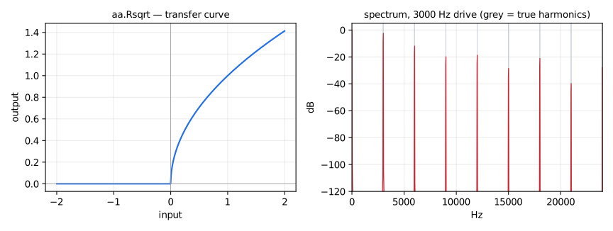
Real-valued sqrt(): a negative input is clamped to 0, so that the output is never NaN.

Usage

Rsqrt(x) : _

Where:

• x: input signal

---

(aa.)Rlog

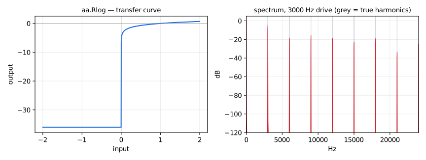
Real-valued log(): the input is clamped to ma.EPSILON from below, so that the output stays finite.

Usage

Rlog(x) : _

Where:

• x: input signal

---

(aa.)Rtan

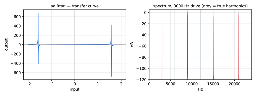
Real-valued tan(): the input is clipped to [-ma.MAX, ma.MAX].

Usage

Rtan(x) : _

Where:

• x: input signal

---

(aa.)Racos

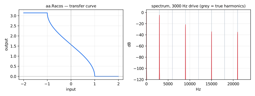
Real-valued acos(): the input is clipped to [-1, 1].

Usage

Racos(x) : _

Where:

• x: input signal

---

(aa.)Rasin

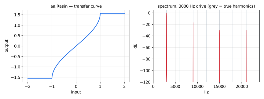
Real-valued asin(): the input is clipped to [-1, 1].

Usage

Rasin(x) : _

Where:

• x: input signal

---

(aa.)Racosh

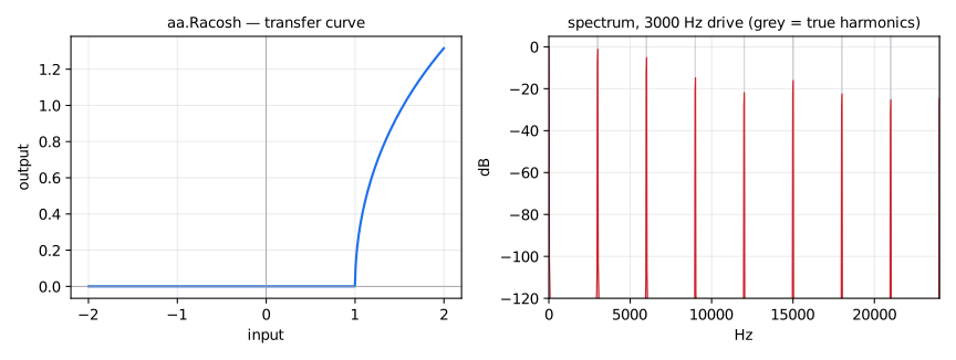
Real-valued acosh(): the input is clipped to [1, ma.MAX].

Usage

Racosh(x) : _

Where:

• x: input signal

---

(aa.)Rcosh

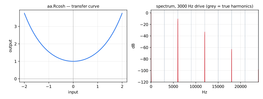
Real-valued cosh(): the output is limited to ma.MAX.

Usage

Rcosh(x) : _

Where:

• x: input signal

---

(aa.)Rsinh

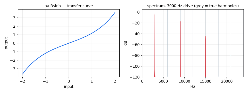
Real-valued sinh(): the output is clipped to [-ma.MAX, ma.MAX].

Usage

Rsinh(x) : _

Where:

• x: input signal

---

(aa.)Ratanh

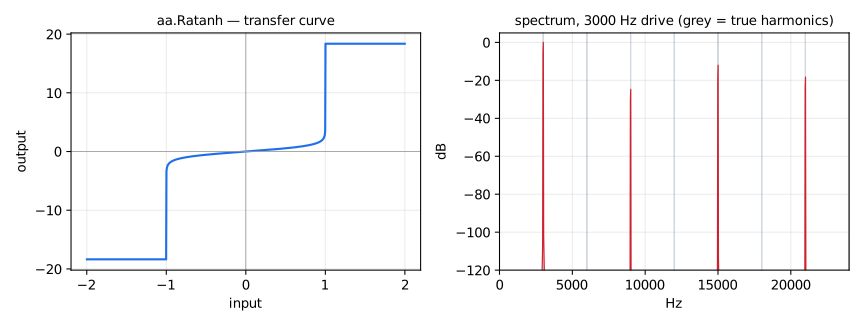
Real-valued atanh(): the input is clipped to [-1 + ma.EPSILON, 1 - ma.EPSILON].

Usage

Ratanh(x) : _

Where:

• x: input signal

---

(aa.)ADAA1

Generalised first-order Antiderivative Anti-Aliasing (ADAA) function.

Implements a first-order ADAA approximation to reduce aliasing in nonlinear audio processing.

Usage

ADAA1(EPS, f, F1, x) : _

Where:

• EPS: a threshold for switching between safe and ill-conditioned paths
• f: a function that we want to process with ADAA
• F1: f's first antiderivative
• x: input signal

Test

aa = library("aanl.lib");
ba = library("basics.lib");
ma = library("maths.lib");
os = library("oscillators.lib");
sig = os.tosc(110);
ADAA1_test = aa.ADAA1(0.001, f, F1, sig)
    with {
        f(x) = max(-1.0, min(1.0, x));
        F1(x) = ba.if((x <= 1.0) & (x >= -1.0), 0.5 * x^2, x * ma.signum(x) - 0.5);
    };

---

(aa.)ADAA2

Generalised second-order Antiderivative Anti-Aliasing (ADAA) function.

Implements a second-order ADAA approximation for even better aliasing reduction at the cost of additional computation.

Usage

ADAA2(EPS, f, F1, F2, x) : _

Where:

• EPS: a threshold for switching between safe and ill-conditioned paths
• f: a function that we want to process with ADAA
• F1: f's first antiderivative
• F2: the antiderivative of x * f(x), as in aa.hardclip2 (not the second antiderivative of f)
• x: input signal

Test

aa = library("aanl.lib");
ba = library("basics.lib");
ma = library("maths.lib");
os = library("oscillators.lib");
sig = os.tosc(110);
ADAA2_test = aa.ADAA2(0.001, f, F1, F2, sig)
    with {
        f(x) = max(-1.0, min(1.0, x));
        F1(x) = ba.if((x <= 1.0) & (x >= -1.0), 0.5 * x^2, x * ma.signum(x) - 0.5);
        F2(x) = ba.if((x <= 1.0) & (x >= -1.0), (1.0 / 3.0) * x^3, ((0.5 * x^2) - 1.0 / 6.0) * ma.signum(x));
    };

Saturators

These antialiased saturators perform best with high-amplitude input signals. If the input is only slightly saturated, hence producing negligible aliasing, the trivial saturator may result in a better overall output, as noise can be introduced by first and second ADAA at low amplitudes.

Once determining the lowest saturation level for which the antialiased functions perform adequately, it might be sensible to cross-fade between the trivial and the antialiased saturators according to the amplitude profile of the input signal.

---

(aa.)hardclip

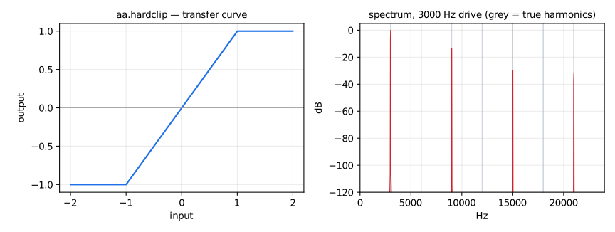
First-order ADAA hard-clip.

The domain of this function is ℝ; its theoretical range is [-1.0; 1.0].

Usage

hardclip(x) : _

Where:

• x: input signal

Test

aa = library("aanl.lib");
os = library("oscillators.lib");
sig = os.tosc(110);
hardclip_test = aa.hardclip(sig);

---

(aa.)hardclip2

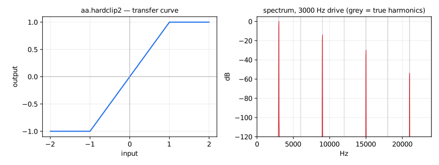
Second-order ADAA hard-clip.

The domain of this function is ℝ; its theoretical range is [-1.0; 1.0].

Usage

hardclip2(x) : _

Where:

• x: input signal

Test

aa = library("aanl.lib");
os = library("oscillators.lib");
sig = os.tosc(110);
hardclip2_test = aa.hardclip2(sig);

---

(aa.)cubic1

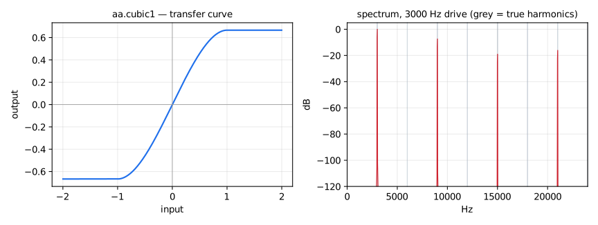
First-order ADAA cubic saturator.

The domain of this function is ℝ; its theoretical range is [-2.0/3.0; 2.0/3.0].

Usage

cubic1(x) : _

Where:

• x: input signal

Test

aa = library("aanl.lib");
os = library("oscillators.lib");
sig = os.tosc(110);
cubic1_test = aa.cubic1(sig);
cubic1_noise_test = aa.cubic1(2.0 * no.noise)
    with { no = library("noises.lib"); };

---

(aa.)parabolic

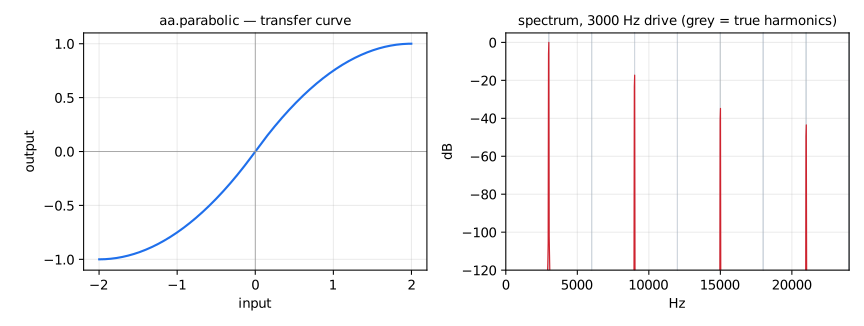
First-order ADAA parabolic saturator.

The domain of this function is ℝ; its theoretical range is [-1.0; 1.0].

Usage

parabolic(x) : _

Where:

• x: input signal

Test

aa = library("aanl.lib");
os = library("oscillators.lib");
sig = os.tosc(110);
parabolic_test = aa.parabolic(sig);
parabolic_noise_test = aa.parabolic(4.0 * no.noise)
    with { no = library("noises.lib"); };

---

(aa.)parabolic2

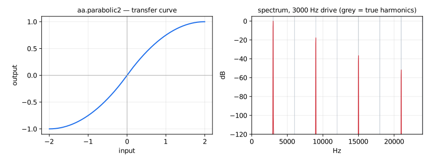
Second-order ADAA parabolic saturator.

The domain of this function is ℝ; its theoretical range is [-1.0; 1.0].

Usage

parabolic2(x) : _

Where:

• x: input signal

Test

aa = library("aanl.lib");
os = library("oscillators.lib");
sig = os.tosc(110);
parabolic2_test = aa.parabolic2(sig);
parabolic2_noise_test = aa.parabolic2(4.0 * no.noise)
    with { no = library("noises.lib"); };

---

(aa.)hyperbolic

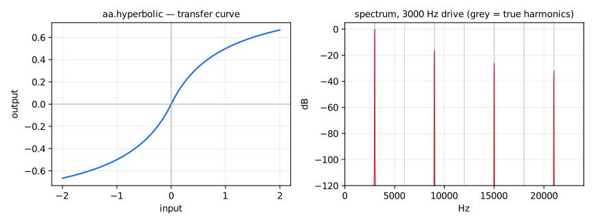
First-order ADAA hyperbolic saturator.

The domain of this function is ℝ; its theoretical range is [-1.0; 1.0].

Usage

hyperbolic(x) : _

Where:

• x: input signal

Test

aa = library("aanl.lib");
os = library("oscillators.lib");
sig = os.tosc(110);
hyperbolic_test = aa.hyperbolic(sig);

---

(aa.)hyperbolic2

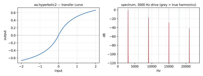
Second-order ADAA hyperbolic saturator.

The domain of this function is ℝ; its theoretical range is [-1.0; 1.0].

Usage

hyperbolic2(x) : _

Where:

• x: input signal

Test

aa = library("aanl.lib");
os = library("oscillators.lib");
sig = os.tosc(110);
hyperbolic2_test = aa.hyperbolic2(sig);

---

(aa.)sinarctan

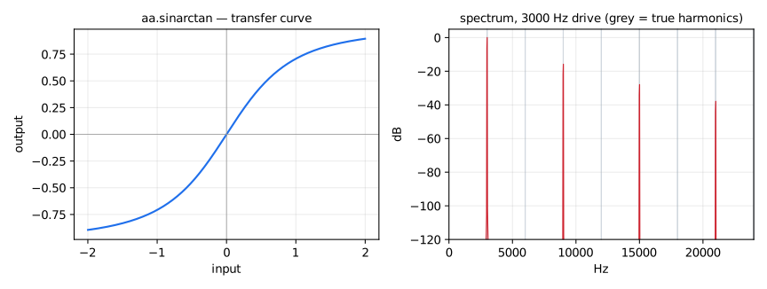
First-order ADAA sin(atan()) saturator.

The domain of this function is ℝ; its theoretical range is [-1.0; 1.0].

Usage

sinarctan(x) : _

Where:

• x: input signal

Test

aa = library("aanl.lib");
os = library("oscillators.lib");
sig = os.tosc(110);
sinarctan_test = aa.sinarctan(sig);

---

(aa.)sinarctan2

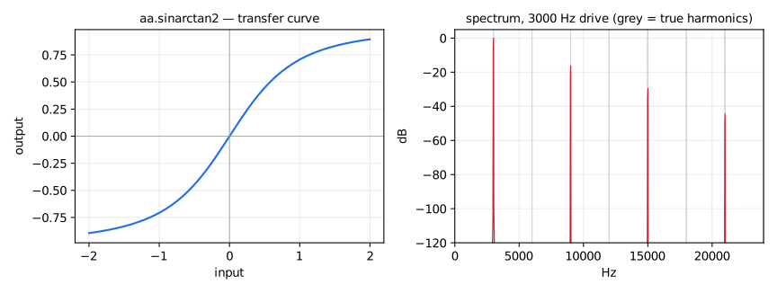
Second-order ADAA sin(atan()) saturator.

The domain of this function is ℝ; its theoretical range is [-1.0; 1.0].

Usage

sinarctan2(x) : _

Where:

• x: input signal

Test

aa = library("aanl.lib");
os = library("oscillators.lib");
sig = os.tosc(110);
sinarctan2_test = aa.sinarctan2(sig);

---

(aa.)sinarctanStable

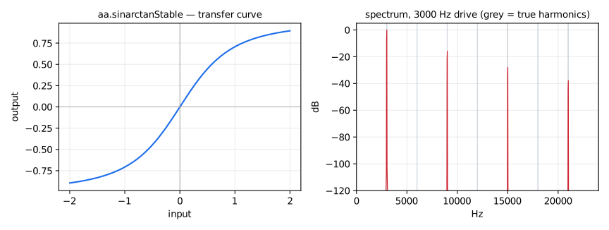
First-order ADAA sin(atan()) saturator, x / sqrt(1 + x^2), evaluated without a threshold or fallback branch.

With F(x) = sqrt(1 + x^2), the difference quotient of aa.sinarctan is rewritten as (x[n] + x[n-1]) / (F(x[n]) + F(x[n-1])), which has no cancellation when x[n] is close to x[n-1] and is exact for any pair of samples. The output is delayed by half a sample, and at Nyquist the linear response is zero, as for any first-order ADAA with a one-sample rectangular kernel. See aa.sinarctanTransparent for a version with a flat linear response.

The domain of this function is ℝ; its theoretical range is [-1.0; 1.0].

Usage

sinarctanStable(x) : _

Where:

• x: input signal

Test

aa = library("aanl.lib");
os = library("oscillators.lib");
sig = os.tosc(110);
sinarctanStable_test = aa.sinarctanStable(5.0 * sig);

References

• M. Vicanek, "Note on Alias Suppression in Digital Distortion", 2023 (revised 2024), eq. (9), https://vicanek.de/articles/AADistortion.pdf

---

(aa.)sinarctanTransparent

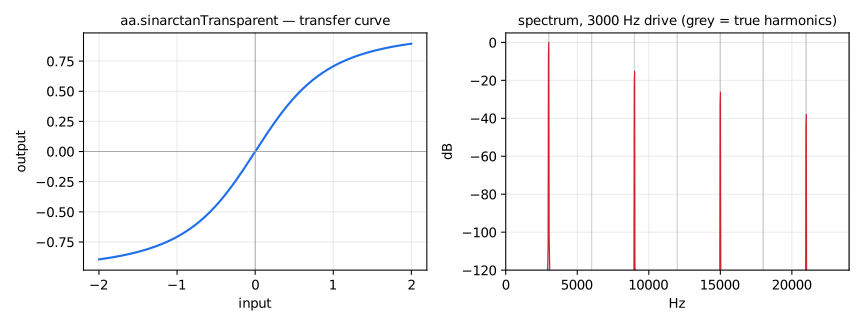
First-order ADAA sin(atan()) saturator, x / sqrt(1 + x^2), with a flat magnitude response in the linear regime.

The rectangular kernel of the antiderivative method is delayed by half a sample, which gives a lowpass of -6 dB at Nyquist (y = (x[n] + 6 x[n-1] + x[n-2]) / 8 for f(x) = x) instead of the zero of the undelayed kernel. The two zeros of that filter are at z = -1 / (3 + sqrt(8)) and its reciprocal, so two identical one-pole filters, y[n] = (1 + a) x[n] - a y[n-1] with a = 1 / (3 + sqrt(8)), one before and one after the shaper, cancel it. Each has unit gain at DC. In the linear regime the whole chain is then the first-order allpass (a + z^-1) / (1 + a z^-1): its magnitude is flat, and its delay is (1 - a) / (1 + a) = 0.71 samples at DC, rising to (1 + a) / (1 - a) = 1.41 samples at Nyquist.

The domain of this function is ℝ; because of the post filter its output can exceed [-1.0; 1.0] by up to about 7 % (a full-scale step peaks at 1.071).

Usage

sinarctanTransparent(x) : _

Where:

• x: input signal

Test

aa = library("aanl.lib");
os = library("oscillators.lib");
sig = os.tosc(110);
sinarctanTransparent_test = aa.sinarctanTransparent(5.0 * sig);

References

• M. Vicanek, "Note on Alias Suppression in Digital Distortion", 2023 (revised 2024), eqs. (4), (6) and (10), https://vicanek.de/articles/AADistortion.pdf

---

(aa.)softclipQuadratic1

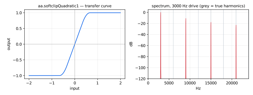
First-order ADAA quadratic softclip.

The domain of this function is ℝ; its theoretical range is [-1.0; 1.0].

Usage

softclipQuadratic1(x) : _

Where:

• x: input signal

Test

aa = library("aanl.lib");
os = library("oscillators.lib");
sig = os.tosc(110);
softclipQuadratic1_test = aa.softclipQuadratic1(sig);

---

(aa.)softclipQuadratic2

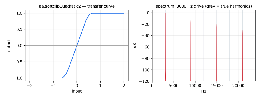
Second-order ADAA quadratic softclip.

The domain of this function is ℝ; its theoretical range is [-1.0; 1.0].

Usage

softclipQuadratic2(x) : _

Where:

• x: input signal

Test

aa = library("aanl.lib");
os = library("oscillators.lib");
sig = os.tosc(110);
softclipQuadratic2_test = aa.softclipQuadratic2(sig);

---

(aa.)tanh1

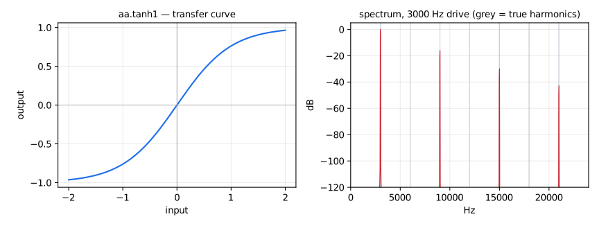
First-order ADAA tanh() saturator.

The domain of this function is ℝ; its theoretical range is [-1.0; 1.0].

Usage

tanh1(x) : _

Where:

• x: input signal

Test

aa = library("aanl.lib");
os = library("oscillators.lib");
sig = os.tosc(110);
tanh1_test = aa.tanh1(sig);

---

(aa.)arctan

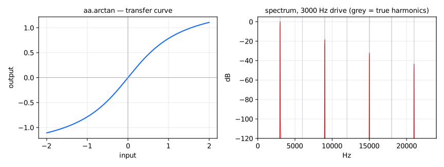
First-order ADAA atan().

The domain of this function is ℝ; its theoretical range is [-π/2.0; π/2.0].

Usage

arctan(x) : _

Where:

• x: input signal

Test

aa = library("aanl.lib");
os = library("oscillators.lib");
sig = os.tosc(110);
arctan_test = aa.arctan(sig);

---

(aa.)arctan2

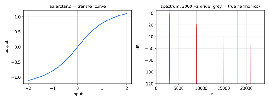
Second-order ADAA atan().

The domain of this function is ℝ; its theoretical range is ]-π/2.0; π/2.0[.

Usage

arctan2(x) : _

Where:

• x: input signal

Test

aa = library("aanl.lib");
os = library("oscillators.lib");
sig = os.tosc(110);
arctan2_test = aa.arctan2(sig);

---

(aa.)asinh1

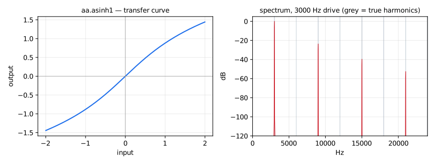
First-order ADAA asinh() saturator (unbounded).

The domain of this function is ℝ; its theoretical range is ℝ.

Usage

asinh1(x) : _

Where:

• x: input signal

Test

aa = library("aanl.lib");
os = library("oscillators.lib");
sig = os.tosc(110);
asinh1_test = aa.asinh1(sig);

---

(aa.)asinh2

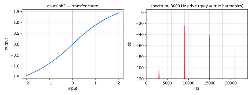
Second-order ADAA asinh() saturator (unbounded).

The domain of this function is ℝ; its theoretical range is ℝ.

Usage

asinh2(x) : _

Where:

• x: input signal

Test

aa = library("aanl.lib");
os = library("oscillators.lib");
sig = os.tosc(110);
asinh2_test = aa.asinh2(sig);

Wavefolders

Wavefolders reflect the part of the signal that exceeds a threshold back towards zero, as many times as needed to keep the output within the threshold. Their slope stays large however hard they are driven, so they alias much more than saturators at the same drive.

The folders below share two parameters: the threshold t and a decay factor r. At each reflection, the part of the input beyond the threshold is scaled by r. With r = 1 the folds are periodic in the input; with r < 1 each fold is 1/r times wider than the previous one, so the output moves more slowly as the input grows. Their antiderivatives are in closed form for any number of folds.

The trivial (non-antialiased) curves are not exported; they are the limit of the ADAA forms for slowly varying inputs.

---

(aa.)triangleFold1

First-order ADAA triangle wavefolder.

The input passes unchanged between -t and t. Beyond, it is reflected back linearly, as many times as needed. With r = 1 this is the classic triangle folder: for |x| > t the output is a triangle wave of the input with period 4t. With r < 1 the excess is scaled by r at every reflection: after k reflections the slope is r^k and the fold is 2t / r^k wide.

The domain of this function is ℝ; its theoretical range is [-t; t].

Usage

triangleFold1(t, r, x) : _

Where:

• t: the threshold, > 0; the output stays within [-t; t] (in single precision, within 1.004 t for inputs up to 20000 t)
• r: the decay factor of the excess at each reflection, in (0; 1]; 1 for periodic folding
• x: input signal

Test

aa = library("aanl.lib");
ba = library("basics.lib");
ma = library("maths.lib");
no = library("noises.lib");
foldSig = 4.0 * no.noise;
foldTri = 1.0 - abs(2.0 * ba.period(P) / P - 1.0) with { P = int(ma.SR / 10); };
triangleFold1_test = aa.triangleFold1(0.5, 0.9, foldSig);
triangleFold1_slider_test = aa.triangleFold1(hslider("t", 0.5, 0.05, 1.0, 0.01), hslider("r", 0.9, 0.5, 1.0, 0.001), foldSig);
triangleFold1_modulated_test = aa.triangleFold1(0.05 + 0.95 * (1.0 - foldTri), 0.5 + 0.5 * foldTri, foldSig);

---

(aa.)triangleFold2

Second-order ADAA triangle wavefolder. Same curve and parameters as aa.triangleFold1.

The domain of this function is ℝ; its theoretical range is [-t; t].

Usage

triangleFold2(t, r, x) : _

Where:

• t: the threshold, > 0; the output stays within [-t; t] in double precision; in single precision it can exceed t once |x| reaches a few thousand times t (up to 1.2 t at 6000 t and 8 t at 20000 t, with t = 0.05 and r = 0.5), by cancellation in the ADAA2 formula
• r: the decay factor of the excess at each reflection, in (0; 1]; 1 for periodic folding
• x: input signal

Test

aa = library("aanl.lib");
ba = library("basics.lib");
ma = library("maths.lib");
no = library("noises.lib");
foldSig = 4.0 * no.noise;
foldTri = 1.0 - abs(2.0 * ba.period(P) / P - 1.0) with { P = int(ma.SR / 10); };
triangleFold2_test = aa.triangleFold2(0.5, 0.9, foldSig);
triangleFold2_slider_test = aa.triangleFold2(hslider("t", 0.5, 0.05, 1.0, 0.01), hslider("r", 0.9, 0.5, 1.0, 0.001), foldSig);
triangleFold2_modulated_test = aa.triangleFold2(0.05 + 0.95 * (1.0 - foldTri), 0.5 + 0.5 * foldTri, foldSig);

---

(aa.)sineFold1

First-order ADAA sine wavefolder.

The input passes unchanged between -t and t. Beyond, each fold is a half-period of a cosine that goes from one threshold to the other, so the slope is 1 inside and 0 at the turning points. With r = 1 the output for |x| > t is t * sin(pi * x / (2t)). With r < 1 each fold is 1/r times wider than the previous one, as for aa.triangleFold1: for |x| > t the output is that of the triangle folder y passed through t * sin(pi * y / (2t)).

The domain of this function is ℝ; its theoretical range is [-t; t].

Usage

sineFold1(t, r, x) : _

Where:

• t: the threshold, > 0; the output stays within [-t; t] (in single precision, within 1.004 t for inputs up to 20000 t)
• r: the decay factor of the fold width, in (0; 1]; 1 for periodic folding
• x: input signal

Test

aa = library("aanl.lib");
ba = library("basics.lib");
ma = library("maths.lib");
no = library("noises.lib");
foldSig = 4.0 * no.noise;
foldTri = 1.0 - abs(2.0 * ba.period(P) / P - 1.0) with { P = int(ma.SR / 10); };
sineFold1_test = aa.sineFold1(0.5, 0.8, foldSig);
sineFold1_slider_test = aa.sineFold1(hslider("t", 0.5, 0.05, 1.0, 0.01), hslider("r", 0.8, 0.5, 1.0, 0.001), foldSig);
sineFold1_modulated_test = aa.sineFold1(0.05 + 0.95 * (1.0 - foldTri), 0.5 + 0.5 * foldTri, foldSig);

---

(aa.)sineFold2

Second-order ADAA sine wavefolder. Same curve and parameters as aa.sineFold1.

The domain of this function is ℝ; its theoretical range is [-t; t].

Usage

sineFold2(t, r, x) : _

Where:

• t: the threshold, > 0; the output stays within [-t; t] in double precision; in single precision it can exceed t once |x| reaches a few thousand times t (up to 1.2 t at 6000 t and 8 t at 20000 t, with t = 0.05 and r = 0.5), by cancellation in the ADAA2 formula
• r: the decay factor of the fold width, in (0; 1]; 1 for periodic folding
• x: input signal

Test

aa = library("aanl.lib");
ba = library("basics.lib");
ma = library("maths.lib");
no = library("noises.lib");
foldSig = 4.0 * no.noise;
foldTri = 1.0 - abs(2.0 * ba.period(P) / P - 1.0) with { P = int(ma.SR / 10); };
sineFold2_test = aa.sineFold2(0.5, 0.8, foldSig);
sineFold2_slider_test = aa.sineFold2(hslider("t", 0.5, 0.05, 1.0, 0.01), hslider("r", 0.8, 0.5, 1.0, 0.001), foldSig);
sineFold2_modulated_test = aa.sineFold2(0.05 + 0.95 * (1.0 - foldTri), 0.5 + 0.5 * foldTri, foldSig);

Trigonometry

These functions are reliable if input signals are within their domains.

---

(aa.)cosine1

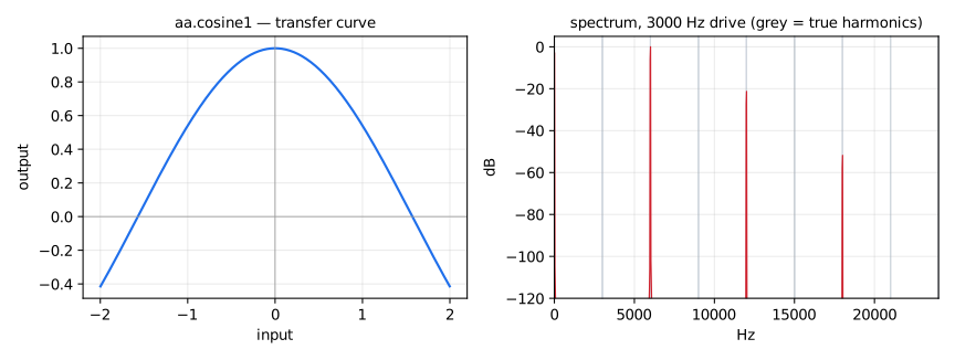
First-order ADAA cos().

The domain of this function is ℝ; its theoretical range is [-1.0; 1.0].

Usage

cosine1(x) : _

Where:

• x: input signal

Test

aa = library("aanl.lib");
os = library("oscillators.lib");
sig = os.tosc(110);
cosine1_test = aa.cosine1(sig);

---

(aa.)cosine2

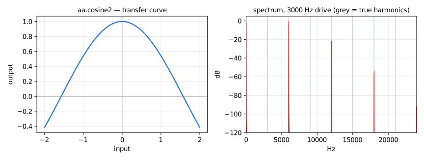
Second-order ADAA cos().

The domain of this function is ℝ; its theoretical range is [-1.0; 1.0].

Usage

cosine2(x) : _

Where:

• x: input signal

Test

aa = library("aanl.lib");
os = library("oscillators.lib");
sig = os.tosc(110);
cosine2_test = aa.cosine2(sig);

---

(aa.)arccos

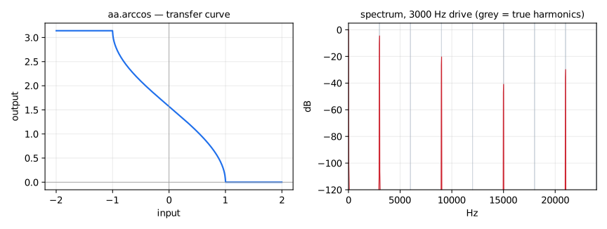
First-order ADAA acos().

The domain of this function is [-1.0; 1.0]; its theoretical range is [π; 0.0].

Usage

arccos(x) : _

Where:

• x: input signal

Test

aa = library("aanl.lib");
os = library("oscillators.lib");
sig = os.tosc(110);
arccos_test = aa.arccos(sig);

---

(aa.)arccos2

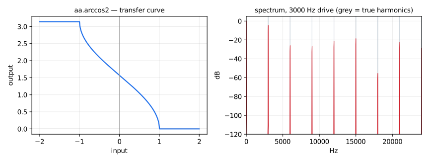
Second-order ADAA acos().

The domain of this function is [-1.0; 1.0]; its theoretical range is [π; 0.0].

Note that this function is not accurate for low-amplitude or low-frequency input signals. In that case, the first-order ADAA arccos() can be used.

Usage

arccos2(x) : _

Where:

• x: input signal

Test

aa = library("aanl.lib");
os = library("oscillators.lib");
sig = os.tosc(110);
arccos2_test = aa.arccos2(sig);
arccos2_noise_test = aa.arccos2(no.noise)
    with { no = library("noises.lib"); };

---

(aa.)acosh1

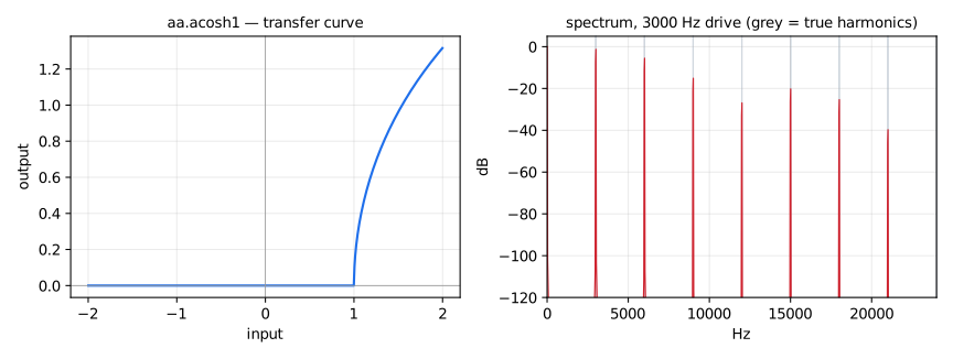
First-order ADAA acosh().

The domain of this function is ℝ >= 1.0; its theoretical range is ℝ >= 0.0.

Usage

acosh1(x) : _

Where:

• x: input signal

Test

aa = library("aanl.lib");
os = library("oscillators.lib");
acoshDomainSig = 1.0 + abs(sig);
sig = os.tosc(110);
acosh1_test = aa.acosh1(acoshDomainSig);

---

(aa.)acosh2

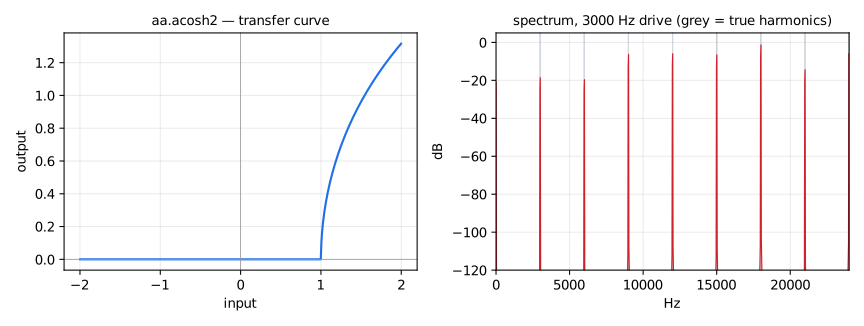
Second-order ADAA acosh().

The domain of this function is ℝ >= 1.0; its theoretical range is ℝ >= 0.0.

Note that this function is not accurate for low-frequency input signals. In that case, the first-order ADAA acosh() can be used.

Usage

acosh2(x) : _

Where:

• x: input signal

Test

aa = library("aanl.lib");
os = library("oscillators.lib");
acoshDomainSig = 1.0 + abs(sig);
sig = os.tosc(110);
acosh2_test = aa.acosh2(acoshDomainSig);

---

(aa.)sine

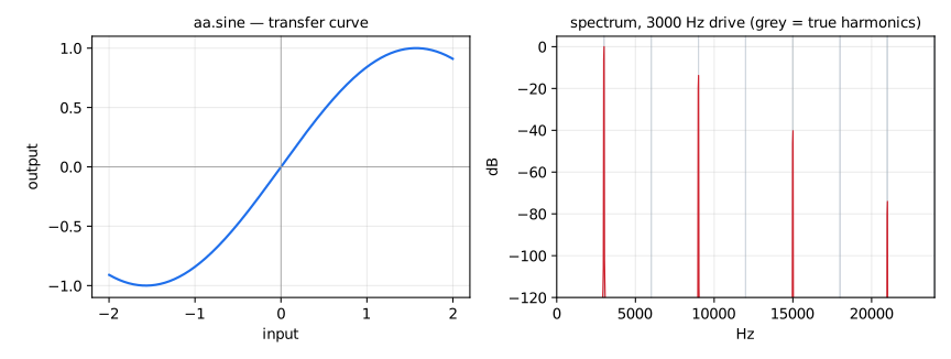
First-order ADAA sin().

The domain of this function is ℝ; its theoretical range is ℝ.

Usage

sine(x) : _

Where:

• x: input signal

Test

aa = library("aanl.lib");
os = library("oscillators.lib");
sig = os.tosc(110);
sine_test = aa.sine(sig);

---

(aa.)sine2

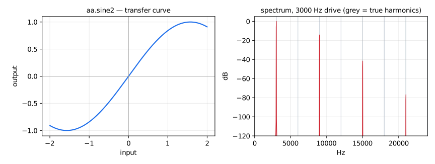
Second-order ADAA sin().

The domain of this function is ℝ; its theoretical range is ℝ.

Usage

sine2(x) : _

Where:

• x: input signal

Test

aa = library("aanl.lib");
os = library("oscillators.lib");
sig = os.tosc(110);
sine2_test = aa.sine2(sig);

---

(aa.)arcsin

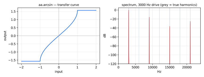
First-order ADAA asin().

The domain of this function is [-1.0, 1.0]; its theoretical range is [-π/2.0; π/2.0].

Usage

arcsin(x) : _

Where:

• x: input signal

Test

aa = library("aanl.lib");
os = library("oscillators.lib");
sig = os.tosc(110);
arcsin_test = aa.arcsin(sig);

---

(aa.)arcsin2

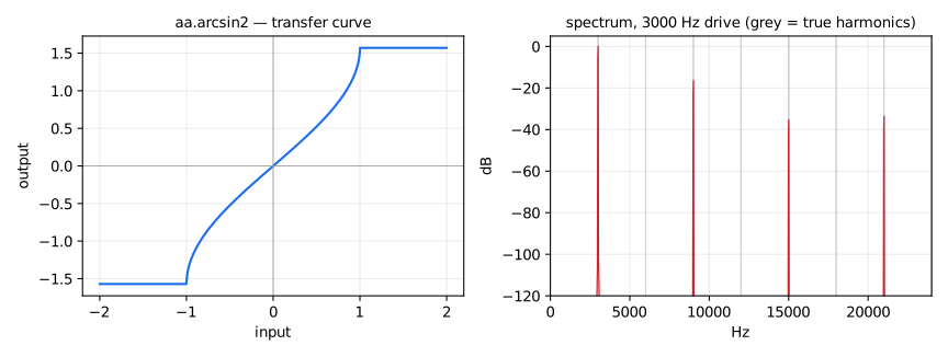
Second-order ADAA asin().

The domain of this function is [-1.0, 1.0]; its theoretical range is [-π/2.0; π/2.0].

Note that this function is not accurate for low-frequency input signals. In that case, the first-order ADAA asin() can be used.

Usage

arcsin2(x) : _

Where:

• x: input signal

Test

aa = library("aanl.lib");
os = library("oscillators.lib");
sig = os.tosc(110);
arcsin2_test = aa.arcsin2(sig);

---

(aa.)tangent

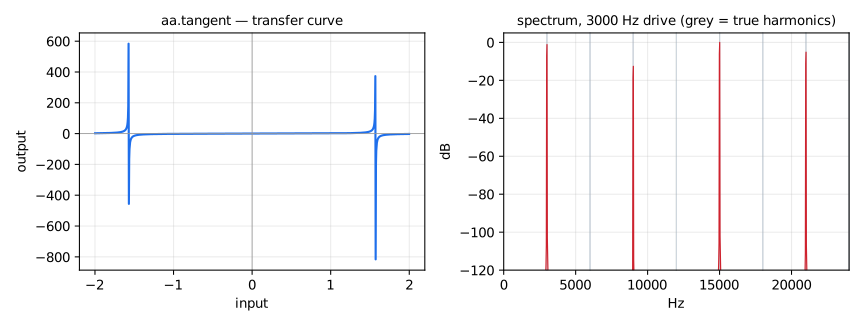
First-order ADAA tan().

The domain of this function is [-π/2.0; π/2.0]; its theoretical range is ℝ.

Usage

tangent(x) : _

Where:

• x: input signal

Test

aa = library("aanl.lib");
ma = library("maths.lib");
os = library("oscillators.lib");
tanDomainSig = 0.25 * ma.PI * sig;
sig = os.tosc(110);
tangent_test = aa.tangent(tanDomainSig);

---

(aa.)atanh1

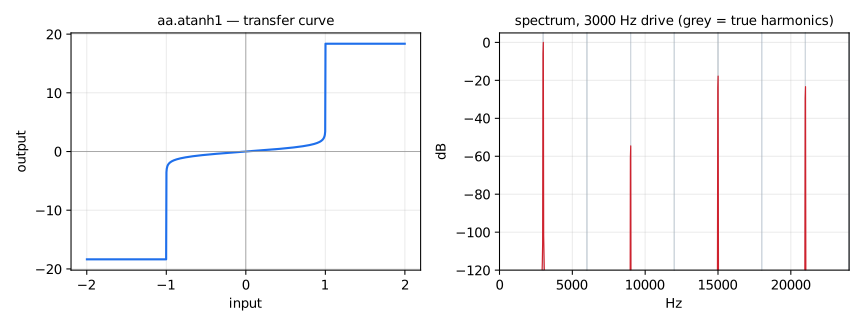
First-order ADAA atanh().

The domain of this function is [-1.0; 1.0]; its theoretical range is ℝ.

Usage

atanh1(x) : _

Where:

• x: input signal

Test

aa = library("aanl.lib");
os = library("oscillators.lib");
atanhDomainSig = 0.8 * sig;
sig = os.tosc(110);
atanh1_test = aa.atanh1(atanhDomainSig);

---

(aa.)atanh2

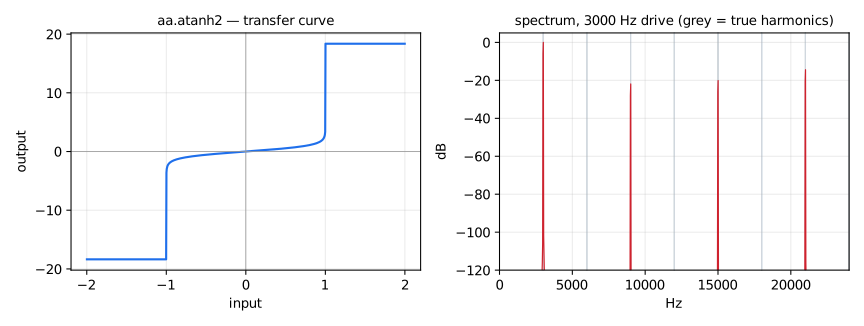
Second-order ADAA atanh().

The domain of this function is [-1.0; 1.0]; its theoretical range is ℝ.

Usage

atanh2(x) : _

Where:

• x: input signal

Test

aa = library("aanl.lib");
os = library("oscillators.lib");
atanhDomainSig = 0.8 * sig;
sig = os.tosc(110);
atanh2_test = aa.atanh2(atanhDomainSig);