
filters.lib
Filters library. Its official prefix is fi.
This library provides a comprehensive collection of linear and nonlinear filters used in audio and signal processing. It includes low-pass, high-pass, band-pass, allpass, shelving, equalizer, and crossover filters, as well as advanced analog and digital filter design sections for both educational and production use.
The Filters library is organized into 25 sections:
- Basic Filters
- Comb Filters
- Direct-Form Digital Filter Sections
- Direct-Form Second-Order Biquad Sections
- Ladder/Lattice Digital Filters
- Useful Special Cases
- Ladder/Lattice Allpass Filters
- Clipping-Prevention Allpass Filters
- Digital Filter Sections Specified as Analog Filter Sections
- Simple Resonator Filters
- Butterworth Lowpass/Highpass Filters
- Special Filter-Bank Delay-Equalizing Allpass Filters
- Elliptic (Cauer) Lowpass Filters
- Elliptic Highpass Filters
- Butterworth Bandpass/Bandstop Filters
- Elliptic Bandpass Filters
- Parametric Equalizers (Shelf, Peaking)
- Mth-Octave Filter-Banks
- Arbitrary-Crossover Filter-Banks and Spectrum Analyzers
- State Variable Filters (SVF)
- Linkwitz-Riley 4th-order 2-way, 3-way, and 4-way crossovers
- Standardized Filters
- Averaging Functions
- Kalman Filters
- Adaptive Filters
References
Basic Filters
(fi.)zero
One zero filter. Difference equation: .
Usage
_ : zero(z) : _
Where:
z: location of zero along real axis in z-plane
Test
fi = library("filters.lib");
os = library("oscillators.lib");
ba = library("basics.lib");
no = library("noises.lib");
ma = library("maths.lib");
src = os.tosc(440);
zero_test = src : fi.zero(0.5);
zero_slider_test = no.noise : fi.zero(hslider("z", 0.5, -1, 1, 0.01));
zero_modulated_test = no.noise : fi.zero(-0.9 + 1.8*tri) with { P = int(ma.SR/10); tri = 1 - abs(2*ba.period(P)/P - 1); };
zero_jump_test = no.noise : fi.zero(-0.9 + 1.8*sq) with { P = int(ma.SR/10); sq = ba.period(2*P) < P; };
References
(fi.)pole
One pole filter. Could also be called a "leaky integrator". Difference equation: .
Usage
_ : pole(p) : _
Where:
p: pole location = feedback coefficient
Test
fi = library("filters.lib");
os = library("oscillators.lib");
ba = library("basics.lib");
no = library("noises.lib");
ma = library("maths.lib");
src = os.tosc(440);
pole_test = src : fi.pole(0.9);
pole_slider_test = no.noise : fi.pole(hslider("p", 0.9, 0, 0.999, 0.001));
pole_modulated_test = no.noise : fi.pole(0.5 + 0.499*tri) with { P = int(ma.SR/10); tri = 1 - abs(2*ba.period(P)/P - 1); };
pole_jump_test = no.noise : fi.pole(0.5 + 0.499*sq) with { P = int(ma.SR/10); sq = ba.period(2*P) < P; };
References
(fi.)integrator
Same as pole(1) [implemented separately for block-diagram clarity].
Usage
_ : integrator : _
Test
fi = library("filters.lib");
os = library("oscillators.lib");
src = os.tosc(440);
integrator_test = src : fi.integrator;
(fi.)dcblockerat
DC blocker with configurable "break frequency".
The amplitude response is substantially flat above fb,
and sloped at about +6 dB/octave below fb.
Derived from the analog transfer function:
(which can be seen as a 1st-order Butterworth highpass filter)
by the low-frequency-matching bilinear transform method
(i.e., using the typical frequency-scaling constant 2*SR).
Usage
_ : dcblockerat(fb) : _
Where:
fb: "break frequency" in Hz, i.e., -3 dB gain frequency (see 2nd reference below)
Test
fi = library("filters.lib");
os = library("oscillators.lib");
ba = library("basics.lib");
no = library("noises.lib");
ma = library("maths.lib");
src = os.tosc(440);
dcblockerat_test = src : fi.dcblockerat(30);
dcblockerat_slider_test = no.noise : fi.dcblockerat(hslider("fb", 30, 1, 500, 1));
dcblockerat_modulated_test = no.noise : fi.dcblockerat(5*pow(40, tri)) with { P = int(ma.SR/10); tri = 1 - abs(2*ba.period(P)/P - 1); };
dcblockerat_jump_test = no.noise : fi.dcblockerat(5*pow(40, sq)) with { P = int(ma.SR/10); sq = ba.period(2*P) < P; };
References
- https://ccrma.stanford.edu/~jos/pasp/Bilinear_Transformation.html
- https://ccrma.stanford.edu/~jos/spectilt/Bode_Plots.html
(fi.)dcblocker
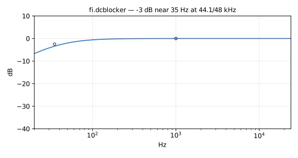
DC blocker. Default dc blocker has -3dB point near 35 Hz (at 44.1 kHz)
and high-frequency gain near 1.0025 (due to no scaling).
dcblocker is a standard Faust function.
Usage
_ : dcblocker : _
Test
fi = library("filters.lib");
os = library("oscillators.lib");
src = os.tosc(440);
dcblocker_test = src : fi.dcblocker;
(fi.)lptN
One-pole lowpass filter with arbitrary dis/charging factors set in dB and times set in seconds.
Usage
_ : lptN(N, tN) : _
Where:
N: is the attenuation factor in dBtN: is the filter period in seconds, that is, the time for the impulse response to decay byNdB
Test
fi = library("filters.lib");
os = library("oscillators.lib");
ba = library("basics.lib");
no = library("noises.lib");
ma = library("maths.lib");
src = os.tosc(440);
lptN_test = src : fi.lptN(60, 0.1);
lptN_slider_test = no.noise : fi.lptN(60, hslider("tN", 0.1, 0.001, 1, 0.001));
lptN_modulated_test = no.noise : fi.lptN(60, 0.001*pow(1000, tri)) with { P = int(ma.SR/10); tri = 1 - abs(2*ba.period(P)/P - 1); };
lptN_jump_test = no.noise : fi.lptN(60, 0.001*pow(1000, sq)) with { P = int(ma.SR/10); sq = ba.period(2*P) < P; };
References
(fi.)lptau
One-pole lowpass with a tau time constant (1/e attenuation after tN seconds).
Usage
_ : lptau(tN) : _
Where:
tN: tau time constant in seconds (1/e attenuation aftertNseconds)
Test
fi = library("filters.lib");
os = library("oscillators.lib");
ba = library("basics.lib");
no = library("noises.lib");
ma = library("maths.lib");
src = os.tosc(440);
lptau_test = src : fi.lptau(0.1);
lptau_slider_test = no.noise : fi.lptau(hslider("tN", 0.1, 0.001, 1, 0.001));
lptau_modulated_test = no.noise : fi.lptau(0.001*pow(1000, tri)) with { P = int(ma.SR/10); tri = 1 - abs(2*ba.period(P)/P - 1); };
lptau_jump_test = no.noise : fi.lptau(0.001*pow(1000, sq)) with { P = int(ma.SR/10); sq = ba.period(2*P) < P; };
(fi.)lpt60
One-pole lowpass with a T60 time constant (60 dB attenuation after tN seconds).
Usage
_ : lpt60(tN) : _
Where:
tN: T60 time constant in seconds (60 dB attenuation aftertNseconds)
Test
fi = library("filters.lib");
os = library("oscillators.lib");
ba = library("basics.lib");
no = library("noises.lib");
ma = library("maths.lib");
src = os.tosc(440);
lpt60_test = src : fi.lpt60(0.3);
lpt60_slider_test = no.noise : fi.lpt60(hslider("tN", 0.3, 0.001, 1, 0.001));
lpt60_modulated_test = no.noise : fi.lpt60(0.001*pow(1000, tri)) with { P = int(ma.SR/10); tri = 1 - abs(2*ba.period(P)/P - 1); };
lpt60_jump_test = no.noise : fi.lpt60(0.001*pow(1000, sq)) with { P = int(ma.SR/10); sq = ba.period(2*P) < P; };
(fi.)lpt19
One-pole lowpass with a T19 time constant (approx. 19 dB attenuation after tN seconds).
Usage
_ : lpt19(tN) : _
Where:
tN: T19 time constant in seconds (approximately 19 dB attenuation aftertNseconds)
Test
fi = library("filters.lib");
os = library("oscillators.lib");
ba = library("basics.lib");
no = library("noises.lib");
ma = library("maths.lib");
src = os.tosc(440);
lpt19_test = src : fi.lpt19(0.2);
lpt19_slider_test = no.noise : fi.lpt19(hslider("tN", 0.2, 0.001, 1, 0.001));
lpt19_modulated_test = no.noise : fi.lpt19(0.001*pow(1000, tri)) with { P = int(ma.SR/10); tri = 1 - abs(2*ba.period(P)/P - 1); };
lpt19_jump_test = no.noise : fi.lpt19(0.001*pow(1000, sq)) with { P = int(ma.SR/10); sq = ba.period(2*P) < P; };
Comb Filters
(fi.)ff_comb
Feed-Forward Comb Filter. Note that ff_comb requires integer delays
(uses delay internally).
ff_comb is a standard Faust function. It computes
y[n] = b0 x[n] + bM x[n - intdel]
Usage
_ : ff_comb(maxdel,intdel,b0,bM) : _
Where:
maxdel: maximum delay (a power of 2)intdel: current (integer) comb-filter delay between 0 and maxdel (a non-integer value is truncated)b0: gain applied to the direct (undelayed) inputbM: gain applied to delay-line output and then summed with the direct path
Test
fi = library("filters.lib");
os = library("oscillators.lib");
ba = library("basics.lib");
no = library("noises.lib");
ma = library("maths.lib");
src = os.tosc(440);
ff_comb_test = src : fi.ff_comb(2048, 64, 1, 0.7);
ff_comb_slider_test = no.noise : fi.ff_comb(2048, hslider("delay", 64, 1, 2047, 1), hslider("b0", 1, -1, 1, 0.01), hslider("bM", 0.7, -1, 1, 0.01));
ff_comb_modulated_test = no.noise : fi.ff_comb(2048, d, 1, 0.7) with { P = int(ma.SR/10); m = 112*(P - abs(2*ba.period(P) - P)); d = 16 + int((m - m % P)/P + 0.5); };
References
(fi.)ff_fcomb
Feed-Forward Comb Filter. Note that ff_fcomb takes floating-point delays
(uses fdelay internally).
ff_fcomb is a standard Faust function. It computes
y[n] = b0 x[n] + bM x[n - del], where x[n - del] is linearly interpolated.
Usage
_ : ff_fcomb(maxdel,del,b0,bM) : _
Where:
maxdel: maximum delay (a power of 2)del: current (float) comb-filter delay between 0 and maxdelb0: gain applied to the direct (undelayed) inputbM: gain applied to delay-line output and then summed with the direct path
Test
fi = library("filters.lib");
os = library("oscillators.lib");
ba = library("basics.lib");
no = library("noises.lib");
ma = library("maths.lib");
src = os.tosc(440);
ff_fcomb_test = src : fi.ff_fcomb(2048, 64.5, 1, 0.7);
ff_fcomb_slider_test = no.noise : fi.ff_fcomb(2048, hslider("delay", 64.5, 1, 2047, 0.01), hslider("b0", 1, -1, 1, 0.01), hslider("bM", 0.7, -1, 1, 0.01));
ff_fcomb_modulated_test = no.noise : fi.ff_fcomb(2048, 16 + 112*tri, 1, 0.7) with { P = int(ma.SR/10); tri = 1 - abs(2*ba.period(P)/P - 1); };
ff_fcomb_jump_test = no.noise : fi.ff_fcomb(2048, 16 + 112*sq, 1, 0.7) with { P = int(ma.SR/10); sq = ba.period(2*P) < P; };
References
(fi.)ffcombfilter
Typical special case of ff_comb() where: b0 = 1.
Usage
_ : ffcombfilter(maxdel,del,g) : _
Where:
maxdel: maximum delay (a power of 2)del: current integer comb-filter delay between 0 and maxdel (a non-integer value is truncated, as inff_comb)g: gain applied to the delayed tap
Test
fi = library("filters.lib");
os = library("oscillators.lib");
ba = library("basics.lib");
no = library("noises.lib");
ma = library("maths.lib");
src = os.tosc(440);
ffcombfilter_test = src : fi.ffcombfilter(2048, 64, 0.7);
ffcombfilter_slider_test = no.noise : fi.ffcombfilter(2048, hslider("delay", 64, 1, 2047, 1), hslider("g", 0.7, -1, 1, 0.01));
ffcombfilter_modulated_test = no.noise : fi.ffcombfilter(2048, d, 0.7) with { P = int(ma.SR/10); m = 112*(P - abs(2*ba.period(P) - P)); d = 16 + int((m - m % P)/P + 0.5); };
(fi.)fb_comb_common
A generic feedback comb filter.
Usage
_ : fb_comb_common(dop,N,b0,aN) : _
Where
dop: delay operator, e.g.@orde.fdelay4a(2048)N: current delayb0: gain applied to inputaN: gain applied to delay-line output
Example test program
process = fb_comb_common(@,N,b0,aN);
implements the following difference equation:
y[n] = b0 x[n] + aN y[n - N]
See more examples in filters.lib below.
Test
fi = library("filters.lib");
os = library("oscillators.lib");
ba = library("basics.lib");
no = library("noises.lib");
ma = library("maths.lib");
src = os.tosc(440);
fb_comb_common_test = src : fi.fb_comb_common(@, 64, 0.8, 0.6);
fb_comb_common_slider_test = no.noise : fi.fb_comb_common(@, hslider("delay", 64, 1, 2047, 1), hslider("b0", 0.8, -1, 1, 0.01), hslider("aN", 0.6, -1, 1, 0.01));
fb_comb_common_modulated_test = no.noise : fi.fb_comb_common(@, d, 0.8, 0.6) with { P = int(ma.SR/10); m = 112*(P - abs(2*ba.period(P) - P)); d = 16 + int((m - m % P)/P + 0.5) : max(16) : min(128); };
(fi.)fb_comb
Feed-Back Comb Filter (integer delay). It computes
y[n] = b0 x[n-1] - aN y[n-del]
The output is delayed by one sample (the mem at the end of the definition):
the transfer function is b0 z^(-1)/(1 + aN z^(-del)), not b0/(1 + aN z^(-del)).
Usage
_ : fb_comb(maxdel,del,b0,aN) : _
Where:
maxdel: maximum delay (a power of 2)del: current integer comb-filter delay (the feedback loop length), between 1 and maxdel (a non-integer value is truncated)b0: input gainaN: minus the gain applied to delay-line output before summing with the input and feeding to the delay line
Test
fi = library("filters.lib");
os = library("oscillators.lib");
ba = library("basics.lib");
no = library("noises.lib");
ma = library("maths.lib");
src = os.tosc(440);
fb_comb_test = src : fi.fb_comb(2048, 64, 0.7, 0.6);
fb_comb_slider_test = no.noise : fi.fb_comb(2048, hslider("delay", 64, 1, 2047, 1), hslider("b0", 0.7, -1, 1, 0.01), hslider("aN", 0.6, -1, 1, 0.01));
fb_comb_modulated_test = no.noise : fi.fb_comb(2048, d, 0.7, 0.6) with { P = int(ma.SR/10); m = 112*(P - abs(2*ba.period(P) - P)); d = 16 + int((m - m % P)/P + 0.5); };
References
(fi.)fb_fcomb
Feed-Back Comb Filter (floating point delay).
fb_fcomb is a standard Faust function. As fb_comb, it computes
y[n] = b0 x[n-1] - aN y[n-del] (the output is delayed by one sample),
where y[n-del] is linearly interpolated.
Usage
_ : fb_fcomb(maxdel,del,b0,aN) : _
Where:
maxdel: maximum delay (a power of 2)del: current (float) comb-filter delay (the feedback loop length), between 1 and maxdelb0: input gainaN: minus the gain applied to delay-line output before summing with the input and feeding to the delay line
Test
fi = library("filters.lib");
os = library("oscillators.lib");
ba = library("basics.lib");
no = library("noises.lib");
ma = library("maths.lib");
src = os.tosc(440);
fb_fcomb_test = src : fi.fb_fcomb(2048, 64.5, 0.7, 0.6);
fb_fcomb_slider_test = no.noise : fi.fb_fcomb(2048, hslider("delay", 64.5, 1, 2047, 0.01), hslider("b0", 0.7, -1, 1, 0.01), hslider("aN", 0.6, -1, 1, 0.01));
fb_fcomb_modulated_test = no.noise : fi.fb_fcomb(2048, 16 + 112*tri, 0.7, 0.6) with { P = int(ma.SR/10); tri = 1 - abs(2*ba.period(P)/P - 1); };
fb_fcomb_jump_test = no.noise : fi.fb_fcomb(2048, 16 + 112*sq, 0.7, 0.6) with { P = int(ma.SR/10); sq = ba.period(2*P) < P; };
References
(fi.)rev1
Special case of fb_comb (rev1(maxdel,N,g) is fb_comb(maxdel,N,1,-g)):
y[n] = x[n-1] + g y[n-N]
The "rev1 section" dates back to the 1960s in computer-music reverberation.
See jcrev and satrev in reverbs.lib for usage examples.
Usage
_ : rev1(maxdel,N,g) : _
Where:
maxdel: maximum delay (a power of 2)N: current feedback comb-filter delay in samples (the loop length, an integer)g: feedback gain
Test
fi = library("filters.lib");
os = library("oscillators.lib");
ba = library("basics.lib");
no = library("noises.lib");
ma = library("maths.lib");
src = os.tosc(440);
rev1_test = src : fi.rev1(2048, 64, 0.6);
rev1_slider_test = no.noise : fi.rev1(2048, hslider("delay", 64, 1, 2047, 1), hslider("g", 0.6, -1, 1, 0.01));
rev1_modulated_test = no.noise : fi.rev1(2048, d, 0.6) with { P = int(ma.SR/10); m = 112*(P - abs(2*ba.period(P) - P)); d = 16 + int((m - m % P)/P + 0.5); };
(fi.)fbcombfilter, (fi.)ffbcombfilter
Other special cases of Feed-Back Comb Filter. Their output is the delay-line output, and the feedback loop is one sample longer than the delay:
y[n] = x[n-intdel] + g y[n-intdel-1]
(with del in place of intdel, linearly interpolated, for ffbcombfilter).
Usage
_ : fbcombfilter(maxdel,del,g) : _
_ : ffbcombfilter(maxdel,del,g) : _
Where:
maxdel: maximum delay (a power of 2)del: current comb-filter delay between 0 and maxdel: an integer forfbcombfilter(usesde.delay; a non-integer value is truncated), a float forffbcombfilter(usesde.fdelay); the loop length isdel+1g: feedback gain
Test
fi = library("filters.lib");
os = library("oscillators.lib");
ba = library("basics.lib");
no = library("noises.lib");
ma = library("maths.lib");
src = os.tosc(440);
fbcombfilter_test = src : fi.fbcombfilter(2048, 64, 0.6);
ffbcombfilter_test = src : fi.ffbcombfilter(2048, 64.5, 0.6);
fbcombfilter_slider_test = no.noise : fi.fbcombfilter(2048, hslider("delay", 64, 1, 2047, 1), hslider("g", 0.6, -1, 1, 0.01));
fbcombfilter_modulated_test = no.noise : fi.fbcombfilter(2048, d, 0.6) with { P = int(ma.SR/10); m = 112*(P - abs(2*ba.period(P) - P)); d = 16 + int((m - m % P)/P + 0.5); };
ffbcombfilter_slider_test = no.noise : fi.ffbcombfilter(2048, hslider("delay", 64.5, 1, 2047, 0.01), hslider("g", 0.6, -1, 1, 0.01));
ffbcombfilter_modulated_test = no.noise : fi.ffbcombfilter(2048, 16 + 112*tri, 0.6) with { P = int(ma.SR/10); tri = 1 - abs(2*ba.period(P)/P - 1); };
ffbcombfilter_jump_test = no.noise : fi.ffbcombfilter(2048, 16 + 112*sq, 0.6) with { P = int(ma.SR/10); sq = ba.period(2*P) < P; };
References
(fi.)allpass_comb
Schroeder Allpass Comb Filter. Note that:
allpass_comb(maxlen,len,aN) : mem = ff_comb(maxlen,len,aN,1) : fb_comb(maxlen,len,1,aN);
(fb_comb delays its output by one sample, hence the mem),
which is a direct-form-1 implementation, requiring two delay lines.
The implementation here is direct-form-2 requiring only one delay line.
Usage
_ : allpass_comb(maxdel,intdel,aN) : _
Where:
maxdel: maximum delay (a power of 2)intdel: current (integer) comb-filter delay between 1 and maxdel (a non-integer value is truncated)aN: minus the feedback gain
Test
fi = library("filters.lib");
os = library("oscillators.lib");
ba = library("basics.lib");
no = library("noises.lib");
ma = library("maths.lib");
src = os.tosc(440);
allpass_comb_test = src : fi.allpass_comb(2048, 64, 0.6);
allpass_comb_slider_test = no.noise : fi.allpass_comb(2048, hslider("delay", 64, 1, 2047, 1), hslider("aN", 0.6, -1, 1, 0.01));
allpass_comb_modulated_test = no.noise : fi.allpass_comb(2048, d, 0.6) with { P = int(ma.SR/10); m = 112*(P - abs(2*ba.period(P) - P)); d = 16 + int((m - m % P)/P + 0.5); };
References
- https://ccrma.stanford.edu/~jos/pasp/Allpass_Two_Combs.html
- https://ccrma.stanford.edu/~jos/pasp/Schroeder_Allpass_Sections.html
- https://ccrma.stanford.edu/~jos/filters/Four_Direct_Forms.html
(fi.)allpass_fcomb
Schroeder Allpass Comb Filter.
allpass_fcomb is a standard Faust function.
Note that:
allpass_fcomb(maxlen,len,aN) : mem = ff_fcomb(maxlen,len,aN,1) : fb_fcomb(maxlen,len,1,aN);
(fb_fcomb delays its output by one sample, hence the mem),
which is a direct-form-1 implementation, requiring two delay lines.
The implementation here is direct-form-2 requiring only one delay line.
The delay line is linearly interpolated (de.fdelay), and linear
interpolation is a lowpass filter at fractional delays, so the response is
allpass only for an integer del. With del = 1000.5 and aN = 0.6, the
impulse response keeps 64% of its energy, and the gain drops by
1.6 dB (8-12 kHz) to 4.3 dB (20-24 kHz) at 48 kHz on average.
allpass_fcomb1a stays allpass at every delay.
Usage
_ : allpass_fcomb(maxdel,del,aN) : _
Where:
maxdel: maximum delay (a power of 2)del: current (float) comb-filter delay between 1 and maxdelaN: minus the feedback gain
Test
fi = library("filters.lib");
os = library("oscillators.lib");
ba = library("basics.lib");
no = library("noises.lib");
ma = library("maths.lib");
src = os.tosc(440);
allpass_fcomb_test = src : fi.allpass_fcomb(2048, 64.5, 0.6);
allpass_fcomb_slider_test = no.noise : fi.allpass_fcomb(2048, hslider("delay", 64.5, 1, 2047, 0.01), hslider("aN", 0.6, -1, 1, 0.01));
allpass_fcomb_modulated_test = no.noise : fi.allpass_fcomb(2048, 16 + 112*tri, 0.6) with { P = int(ma.SR/10); tri = 1 - abs(2*ba.period(P)/P - 1); };
allpass_fcomb_jump_test = no.noise : fi.allpass_fcomb(2048, 16 + 112*sq, 0.6) with { P = int(ma.SR/10); sq = ba.period(2*P) < P; };
References
- https://ccrma.stanford.edu/~jos/pasp/Allpass_Two_Combs.html
- https://ccrma.stanford.edu/~jos/pasp/Schroeder_Allpass_Sections.html
- https://ccrma.stanford.edu/~jos/filters/Four_Direct_Forms.html
(fi.)rev2
Special case of allpass_comb (rev2(maxlen,len,g)).
The "rev2 section" dates back to the 1960s in computer-music reverberation.
See jcrev and satrev in reverbs.lib for usage examples.
Usage
_ : rev2(maxlen,len,g) : _
Where:
maxlen: maximum delay (a power of 2)len: current allpass comb-filter delay in samplesg: allpass coefficient (its sign is negated internally)
Test
fi = library("filters.lib");
os = library("oscillators.lib");
ba = library("basics.lib");
no = library("noises.lib");
ma = library("maths.lib");
src = os.tosc(440);
rev2_test = src : fi.rev2(2048, 64, 0.6);
rev2_slider_test = no.noise : fi.rev2(2048, hslider("delay", 64, 1, 2047, 1), hslider("g", 0.6, -1, 1, 0.01));
rev2_modulated_test = no.noise : fi.rev2(2048, d, 0.6) with { P = int(ma.SR/10); m = 112*(P - abs(2*ba.period(P) - P)); d = 16 + int((m - m % P)/P + 0.5); };
(fi.)allpass_fcomb5, (fi.)allpass_fcomb1a
Same as allpass_fcomb but use fdelay5 and fdelay1a internally
(Interpolation helps - look at an fft of faust2octave on:
1-1' <: allpass_fcomb(1024,10.5,0.95), allpass_fcomb5(1024,10.5,0.95);)
allpass_fcomb1a (first-order Thiran allpass interpolation) is allpass at
every delay N from 1.5 to maxdel. allpass_fcomb5 (fifth-order Lagrange
interpolation) is allpass only for an integer N: at fractional delays the
interpolator is a lowpass filter, worst at a fractional part of 0.5. With
N = 1000.5 and aN = 0.6, the impulse response keeps 79% of its energy:
the gain is within 0.2 dB of unity up to SR/4 on average, and drops by
2.5 dB (16-20 kHz) to 4 dB (20-24 kHz) at 48 kHz.
allpass_fcomb5 needs N from 3 to maxdel-1: above maxdel-1 the top
interpolator tap is clamped by the delay line, and the gain exceeds unity
(by up to 0.28 dB at N = 2047.5 with maxdel = 2048).
Usage
_ : allpass_fcomb5(maxdel,N,aN) : _
_ : allpass_fcomb1a(maxdel,N,aN) : _
Where:
maxdel: maximum delay (a power of 2)N: current (float) allpass comb-filter delay between 0 and maxdelaN: allpass coefficient: the transfer function is (aN + z^(-N))/(1 + aN z^(-N))
Test
fi = library("filters.lib");
os = library("oscillators.lib");
ba = library("basics.lib");
no = library("noises.lib");
ma = library("maths.lib");
src = os.tosc(440);
allpass_fcomb5_test = src : fi.allpass_fcomb5(2048, 64.5, 0.6);
allpass_fcomb1a_test = src : fi.allpass_fcomb1a(2048, 64.5, 0.6);
allpass_fcomb5_slider_test = no.noise : fi.allpass_fcomb5(2048, hslider("delay", 64.5, 1, 2047, 0.01), hslider("aN", 0.6, -1, 1, 0.01));
allpass_fcomb5_modulated_test = no.noise : fi.allpass_fcomb5(2048, 16 + 112*tri, 0.6) with { P = int(ma.SR/10); tri = 1 - abs(2*ba.period(P)/P - 1); };
allpass_fcomb5_jump_test = no.noise : fi.allpass_fcomb5(2048, 16 + 112*sq, 0.6) with { P = int(ma.SR/10); sq = ba.period(2*P) < P; };
allpass_fcomb1a_slider_test = no.noise : fi.allpass_fcomb1a(2048, hslider("delay", 64.5, 1, 2047, 0.01), hslider("aN", 0.6, -1, 1, 0.01));
allpass_fcomb1a_modulated_test = no.noise : fi.allpass_fcomb1a(2048, 16 + 112*tri, 0.6) with { P = int(ma.SR/10); tri = 1 - abs(2*ba.period(P)/P - 1); };
allpass_fcomb1a_jump_test = no.noise : fi.allpass_fcomb1a(2048, 16 + 112*sq, 0.6) with { P = int(ma.SR/10); sq = ba.period(2*P) < P; };
Direct-Form Digital Filter Sections
Filters specified by transfer-function polynomials B(z)/A(z), computed
directly from their coefficients. A direct form loses precision when its
poles come close to z = 1, that is, for frequencies low relative to the
sample rate, and it behaves badly when its coefficients change while it
runs. For an analog prototype, prefer the functions of the section
Digital Filter Sections Specified as Analog Filter Sections,
whose references explain why. For a second-order z-domain design whose
coefficients move, tf2_tpt realizes the same B(z)/A(z) as a
state-variable filter.
(fi.)iir
Nth-order Infinite-Impulse-Response (IIR) digital filter, implemented in terms of the Transfer-Function (TF) coefficients. Such filter structures are termed "direct form".
iir is a standard Faust function.
Usage
_ : iir(bcoeffs,acoeffs) : _
Where:
bcoeffs: (b0,b1,...,b_order) = TF numerator coefficientsacoeffs: (a1,...,a_order) = TF denominator coeffs (a0=1)
Test
fi = library("filters.lib");
os = library("oscillators.lib");
src = os.tosc(440);
iir_test = src : fi.iir((0.5, 0.5), (0.3));
References
(fi.)fir
FIR filter (convolution of FIR filter coefficients with a signal).
fir is a standard Faust function.
Usage
_ : fir(bv) : _
Where:
bv:b0,b1,...,bn, a parallel bank of coefficient signals
Note
bv is processed using pattern-matching at compile time,
so it must have this normal form (parallel signals).
Example test program
Smoothing white noise with a five-point moving average:
bv = .2,.2,.2,.2,.2;
process = noise : fir(bv);
Equivalent (note double parens):
process = noise : fir((.2,.2,.2,.2,.2));
Test
fi = library("filters.lib");
os = library("oscillators.lib");
src = os.tosc(440);
fir_test = src : fi.fir((0.2, 0.2, 0.2, 0.2, 0.2));
(fi.)conv, (fi.)convN
Convolution of input signal with given coefficients. conv filters one
signal with all the coefficients. convN takes N signals and sums the i-th,
delayed by i samples, times the i-th coefficient: split one signal to N
copies first to convolve it with the first N coefficients.
Usage
_ : conv(kv) : _
si.bus(N) : convN(N,kv) : _ // Useful when N < ba.count(kv)
_ <: si.bus(N) : convN(N,kv) : _ // one signal, N coefficients
Where:
kv: the list of coefficients(k1,k2,k3,...), one signal bankN: number of input signals ofconvN, at most the number of coefficients (a constant numerical expression)
Example
_ : conv((0.25,0.25,0.25,0.25)) : _
_ <: si.bus(3) : convN(3,(0.3,0.2,0.1,0.05)) : _
Test
fi = library("filters.lib");
os = library("oscillators.lib");
si = library("signals.lib");
src = os.tosc(440);
convN_test = (src <: si.bus(3)) : fi.convN(3, (0.3, 0.2, 0.1, 0.05));
conv_test = src : fi.conv((0.25, 0.25, 0.25, 0.25));
(fi.)tf1, (fi.)tf2, (fi.)tf3
tfN = N'th-order direct-form digital filter.
tf2 is a standard Faust function.
Usage
_ : tf1(b0,b1,a1) : _
_ : tf2(b0,b1,b2,a1,a2) : _
_ : tf3(b0,b1,b2,b3,a1,a2,a3) : _
Where:
b0,b1,b2,b3: transfer-function numerator coefficients (b0..bNfortfN)a1,a2,a3: transfer-function denominator coefficients, the denominator being monic (a0 = 1;a1..aNfortfN)
Test
fi = library("filters.lib");
os = library("oscillators.lib");
src = os.tosc(440);
tf1_test = src : fi.tf1(0.5, 0.25, -0.4);
tf2_test = src : fi.tf2(0.1, 0.2, 0.1, -0.5, 0.06);
tf3_test = src : fi.tf3(0.1, 0.3, 0.3, 0.1, -0.9, 0.26, -0.024);
References
(fi.)TF2
Tunable second-order direct-form digital filter, the "original"
biquad of music.lib: y[n] = b0x[n] + b1x[n-1] + b2x[n-2] -
a1y[n-1] - a2*y[n-2]. Kept for comparison and for the compatibility
libraries (maxmsp.lib, instruments.lib); new code should use tf2
instead.
Usage
_ : TF2(b0,b1,b2,a1,a2) : _
Where:
b0,b1,b2: the feedforward coefficientsa1,a2: the feedback coefficients
Test
fi = library("filters.lib");
os = library("oscillators.lib");
TF2_legacy_test = os.tosc(440) : fi.TF2(0.2, 0.4, 0.2, -0.5, 0.3);
(fi.)tf2_tpt
Second-order digital filter N(z)/A(z), with A(z) = 1 + a1 z^-1 + a2 z^-2
and N(z) = n0 + n1 z^-1 + n2 z^-2, realized as a trapezoidal
(topology-preserving) state-variable filter with exactly the same poles and
zeros. It is for z-domain designs whose parameters move (a pole radius and
angle, a notch or allpass frequency): the same filter as tf2, but it stays
accurate in single precision when the poles approach z = 1 or z = -1, and
its output stays continuous when the coefficients jump or move at audio
rate, where a direct form rings or diverges. For an analog prototype, use
tf2s.
The coefficients are passed in a form the caller computes without
cancellation from its design parameters, never from rounded a1 and a2
(see the method below).
Usage
_ : tf2_tpt(P,S,fq,Np,Nm,nd) : _
Where:
P:A(1) = 1 + a1 + a2, positive, or 0 together withNp(a pole and a zero at z = 1 that cancel, as innotchwat 0 Hz)S:A(-1) = 1 - a1 + a2, positive, or 0 together withNm(a pole and a zero at z = -1 that cancel, as innotchwat the Nyquist limit)fq:1 - a2, positive (P + S + 2*fq = 4)Np:N(1) = n0 + n1 + n2, the gain at DC isNp/PNm:N(-1) = n0 - n1 + n2, the gain at Nyquist isNm/Snd:n0 - n2
Method
For complex poles r*exp(+-j*th), with om = 1 - r computed directly
(for example 0 - ma.expm1(-PI*B/SR) for a bandwidth B):
P = om^2 + 4*r*sin(th/2)^2, S = om^2 + 4*r*cos(th/2)^2 and
fq = om*(2 - om). Near the Nyquist limit, compute cos(th/2) as
sin(PI*(SR/2 - f)/SR) for a frequency f, so that S is as accurate as
P. For example, a resonator of unity peak gain,
(1 - r^2)/2*(1 - z^-2)/A(z), is tf2_tpt(P,S,fq,0,0,fq), and the notch
(1 + A_ap(z))/2 of an allpass A_ap with these poles is
tf2_tpt(P,S,fq,P,S,0) (see notchw).
The state-variable filter has g = sqrt(P/S), k*g = 2*fq/S and
1 + k*g + g^2 = 4/S, and its highpass, bandpass and lowpass outputs map
onto the numerator with the taps cH = Nm/S, cB = 2*nd/(g*S) and
cL = Np/P. Since hp + k*bp + lp = x, the output is computed as
cH*x + (cB - k*cH)*bp + (cL - cH)*lp, and the state-variable filter runs
on x scaled by the larger of the last two taps, so that its states hold the
dominant part of the output at the output level. Each coefficient update
costs four divisions and one square root; none per sample when the
coefficients are constant.
When P > S (poles with Re z < 0: a resonance above SR/4), the section
is mirrored: it realizes H(z) = H'(-z), where H' has P and S, and
Np and Nm, exchanged, by replacing each state delay z^-1 with -z^-1
(under the bilinear transform, z -> -z is s -> 1/s). The poles of H' have
Re z > 0 and g <= 1, so a pole near z = -1 is as accurate as one near
z = 1. When the coefficients cross P = S, the states are mapped to those
of the other form that give the same output.
Test
fi = library("filters.lib");
ba = library("basics.lib");
ma = library("maths.lib");
no = library("noises.lib");
os = library("oscillators.lib");
tf2_tpt_test = no.noise : fi.tf2_tpt(P, S, fq, 0, 0, fq) with { fc = 1000; om = 0 - ma.expm1(0 - ma.PI*fc/10/ma.SR); r = 1 - om; th = 2*ma.PI*fc/ma.SR; P = om*om + 4*r*sin(0.5*th)^2; S = om*om + 4*r*cos(0.5*th)^2; fq = om*(2 - om); };
tf2_tpt_slider_test = no.noise : fi.tf2_tpt(P, S, fq, 0, 0, fq) with { fc = hslider("fc", 1000, 20, 20000, 1); om = 0 - ma.expm1(0 - ma.PI*fc/10/ma.SR); r = 1 - om; th = 2*ma.PI*fc/ma.SR; P = om*om + 4*r*sin(0.5*th)^2; S = om*om + 4*r*cos(0.5*th)^2; fq = om*(2 - om); };
tf2_tpt_modulated_test = no.noise : fi.tf2_tpt(P, S, fq, 0, 0, fq) with { Pd = int(ma.SR/10); tri = 1 - abs(2*ba.period(Pd)/Pd - 1); fc = 20*pow(250, tri); om = 0 - ma.expm1(0 - ma.PI*fc/10/ma.SR); r = 1 - om; th = 2*ma.PI*fc/ma.SR; P = om*om + 4*r*sin(0.5*th)^2; S = om*om + 4*r*cos(0.5*th)^2; fq = om*(2 - om); };
tf2_tpt_jump_test = no.noise : fi.tf2_tpt(P, S, fq, 0, 0, fq) with { Pd = int(ma.SR/10); sq = ba.period(2*Pd) < Pd; fc = 20*pow(250.0, sq); om = 0 - ma.expm1(0 - ma.PI*fc/10/ma.SR); r = 1 - om; th = 2*ma.PI*fc/ma.SR; P = om*om + 4*r*sin(0.5*th)^2; S = om*om + 4*r*cos(0.5*th)^2; fq = om*(2 - om); };
tf2_tpt_audio_modulated_test = 0.1*no.noise : fi.tf2_tpt(P, S, fq, 0, 0, fq) with { fc = max(20, 1000*(1 + 0.9*os.tosc(500))); om = 0 - ma.expm1(0 - ma.PI*fc/10/ma.SR); r = 1 - om; th = 2*ma.PI*fc/ma.SR; P = om*om + 4*r*sin(0.5*th)^2; S = om*om + 4*r*cos(0.5*th)^2; fq = om*(2 - om); };
tf2_tpt_high_test = no.noise : fi.tf2_tpt(P, S, fq, 0, 0, fq) with { fc = ma.SR/2 - 200; om = 0 - ma.expm1(0 - ma.PI*100/ma.SR); r = 1 - om; P = om*om + 4*r*sin(ma.PI*fc/ma.SR)^2; S = om*om + 4*r*sin(ma.PI*(0.5*ma.SR - fc)/ma.SR)^2; fq = om*(2 - om); };
tf2_tpt_mirror_modulated_test = no.noise : fi.tf2_tpt(P, S, fq, 0, 0, fq) with { Pd = int(ma.SR/10); tri = 1 - abs(2*ba.period(Pd)/Pd - 1); fc = ma.SR*(0.1 + 0.35*tri); om = 0 - ma.expm1(0 - ma.PI*fc/10/ma.SR); r = 1 - om; P = om*om + 4*r*sin(ma.PI*fc/ma.SR)^2; S = om*om + 4*r*sin(ma.PI*(0.5*ma.SR - fc)/ma.SR)^2; fq = om*(2 - om); };
tf2_tpt_mirror_jump_test = no.noise : fi.tf2_tpt(P, S, fq, 0, 0, fq) with { Pd = int(ma.SR/10); sq = ba.period(2*Pd) < Pd; fc = ma.SR*select2(sq, 0.1, 0.45); om = 0 - ma.expm1(0 - ma.PI*fc/10/ma.SR); r = 1 - om; P = om*om + 4*r*sin(ma.PI*fc/ma.SR)^2; S = om*om + 4*r*sin(ma.PI*(0.5*ma.SR - fc)/ma.SR)^2; fq = om*(2 - om); };
References
- Julius O. Smith III, "Digital State-Variable Filters": https://ccrma.stanford.edu/~jos/svf/
- Vadim Zavalishin, "The Art of VA Filter Design", revision 2.1.2, 2020: https://www.discodsp.net/VAFilterDesign_2.1.2.pdf
(fi.)notchw
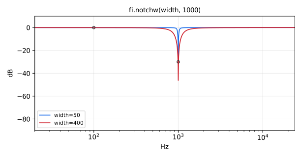
Simple notch filter based on a biquad, realized with tf2_tpt.
notchw is a standard Faust function.
Usage:
_ : notchw(width,freq) : _
Where:
width: "notch width" in Hz (approximate)freq: "notch frequency" in Hz, from 0 (a first-order DC notch) toma.SR/2(a first-order notch at the Nyquist limit). Abovema.SR/4the section runs mirrored (seetf2_tpt), so that a notch near the Nyquist limit is as accurate as one near 0 Hz
Test
fi = library("filters.lib");
os = library("oscillators.lib");
ba = library("basics.lib");
no = library("noises.lib");
ma = library("maths.lib");
src = os.tosc(440);
notchw_test = src : fi.notchw(200, 1000);
notchw_slider_test = no.noise : fi.notchw(hslider("width", 200, 10, 2000, 1), hslider("freq", 1000, 20, 20000, 1));
notchw_modulated_test = no.noise : fi.notchw(100, 200*pow(25, tri)) with { P = int(ma.SR/10); tri = 1 - abs(2*ba.period(P)/P - 1); };
notchw_jump_test = no.noise : fi.notchw(100, 200*pow(25, sq)) with { P = int(ma.SR/10); sq = ba.period(2*P) < P; };
notchw_audio_modulated_test = 0.1*no.noise : fi.notchw(fc/10, fc) with { fc = max(20, 1000*(1 + 0.9*os.tosc(500))); };
notchw_dc_test = no.noise : fi.notchw(100, 0);
notchw_nyquist_test = no.noise : fi.notchw(100, ma.SR/2);
notchw_high_test = no.noise : fi.notchw(100, ma.SR/2 - 100);
notchw_mirror_modulated_test = no.noise : fi.notchw(1000, ma.SR*(0.1 + 0.35*tri)) with { P = int(ma.SR/10); tri = 1 - abs(2*ba.period(P)/P - 1); };
notchw_mirror_jump_test = no.noise : fi.notchw(1000, ma.SR*select2(sq, 0.1, 0.45)) with { P = int(ma.SR/10); sq = ba.period(2*P) < P; };
References
- https://ccrma.stanford.edu/~jos/pasp/Phasing_2nd_Order_Allpass_Filters.html
- Julius O. Smith III, "Digital State-Variable Filters", for the trapezoidal
(TPT) state-variable filter that
tf2_tptruns on: https://ccrma.stanford.edu/~jos/svf/
Direct-Form Second-Order Biquad Sections
Direct-Form Second-Order Biquad Sections
References
(fi.)tf21, (fi.)tf22, (fi.)tf22t, (fi.)tf21t
tfN = N'th-order direct-form digital filter where:
tf21is tf2, direct-form 1tf22is tf2, direct-form 2tf22tis tf2, direct-form 2 transposedtf21tis tf2, direct-form 1 transposed
Usage
_ : tf21(b0,b1,b2,a1,a2) : _
_ : tf22(b0,b1,b2,a1,a2) : _
_ : tf22t(b0,b1,b2,a1,a2) : _
_ : tf21t(b0,b1,b2,a1,a2) : _
Where:
b0,b1,b2: transfer-function numerator coefficientsa1,a2: transfer-function denominator coefficients (monic denominator,a0 = 1)
Test
fi = library("filters.lib");
os = library("oscillators.lib");
src = os.tosc(440);
tf21_test = src : fi.tf21(0.1, 0.2, 0.1, -0.5, 0.06);
tf22_test = src : fi.tf22(0.1, 0.2, 0.1, -0.5, 0.06);
tf22t_test = src : fi.tf22t(0.1, 0.2, 0.1, -0.5, 0.06);
tf21t_test = src : fi.tf21t(0.1, 0.2, 0.1, -0.5, 0.06);
References
Ladder/Lattice Digital Filters
Ladder and lattice digital filters generally have superior numerical properties relative to direct-form digital filters. They can be derived from digital waveguide filters, which gives them a physical interpretation.
References
- F. Itakura and S. Saito: "Digital Filtering Techniques for Speech Analysis and Synthesis", 7th Int. Cong. Acoustics, Budapest, 25 C 1, 1971.
- J. D. Markel and A. H. Gray: Linear Prediction of Speech, New York: Springer Verlag, 1976.
- https://ccrma.stanford.edu/~jos/pasp/Conventional_Ladder_Filters.html
(fi.)av2sv
Compute reflection coefficients sv from transfer-function denominator av.
The output sv is the parallel signal bank s1,...,sN, where si is
the i'th reflection coefficient.
Usage
av2sv(av) : si.bus(ba.count(av))
Where:
av: parallel signal banka1,...,aN, whereaiis the coefficient ofz^(-i)in the filter transfer-function denominatorA(z)
Test
fi = library("filters.lib");
si = library("signals.lib");
av2sv_test = fi.av2sv((-0.4, 0.1)) : si.bus(2);
References
https://ccrma.stanford.edu/~jos/filters/Step_Down_Procedure.html (where reflection coefficients are denoted by k rather than s).
(fi.)bvav2nuv
Compute lattice tap coefficients from transfer-function coefficients.
The output nuv is the parallel signal bank nu0,nu1,...,nuN (N+1
signals), where nui is the i'th tap coefficient.
Usage
bvav2nuv(bv,av) : si.bus(ba.count(av)+1)
Where:
bv: parallel signal bankb0,b1,...,bN, wherebiis the coefficient ofz^(-i)in the filter numeratorav: parallel signal banka1,...,aN, whereaiis the coefficient ofz^(-i)in the filter denominator
Test
fi = library("filters.lib");
si = library("signals.lib");
bvav2nuv_test = fi.bvav2nuv((0.1, 0.2, 0.3), (-0.4, 0.1)) : si.bus(3);
(fi.)iir_lat2
Two-multiply lattice IIR filter of arbitrary order.
Usage
_ : iir_lat2(bv,av) : _
Where:
bv: transfer-function numeratorav: transfer-function denominator (monic)
Test
fi = library("filters.lib");
os = library("oscillators.lib");
src = os.tosc(440);
iir_lat2_test = src : fi.iir_lat2((0.1, 0.2, 0.3), (-0.4, 0.1));
(fi.)allpassnt
Two-multiply lattice allpass (nested order-1 direct-form-ii allpasses), with taps.
Usage
_ : allpassnt(n,sv) : si.bus(n+1)
Where:
n: the order of the filtersv: the reflection coefficients (-1 1)
The first output is the n-th order allpass output, while the remaining outputs are taps taken from the input of each delay element from the input to the output. See (fi.)allpassn for the single-output case.
Test
fi = library("filters.lib");
os = library("oscillators.lib");
si = library("signals.lib");
src = os.tosc(440);
allpassnt_test = src : fi.allpassnt(2, (0.3, -0.2)) : si.bus(3);
(fi.)iir_kl
Kelly-Lochbaum ladder IIR filter of arbitrary order.
Usage
_ : iir_kl(bv,av) : _
Where:
bv: transfer-function numeratorav: transfer-function denominator (monic)
Test
fi = library("filters.lib");
os = library("oscillators.lib");
src = os.tosc(440);
iir_kl_test = src : fi.iir_kl((0.1, 0.2, 0.3), (-0.4, 0.1));
(fi.)allpassnklt
Kelly-Lochbaum ladder allpass. Its n+1 outputs are the allpass output
followed by the n tap signals of the ladder (used by iir_kl to form
a general transfer function).
Usage:
_ : allpassnklt(n,sv) : si.bus(n+1)
Where:
n: the order of the filtersv: the reflection coefficients (-1 1)
Test
fi = library("filters.lib");
os = library("oscillators.lib");
si = library("signals.lib");
src = os.tosc(440);
allpassnklt_test = src : fi.allpassnklt(2, (0.3, -0.2)) : si.bus(3);
(fi.)iir_lat1
One-multiply lattice IIR filter of arbitrary order.
Usage
_ : iir_lat1(bv,av) : _
Where:
bv: transfer-function numerator as a bank of parallel signalsav: transfer-function denominator as a bank of parallel signals
Test
fi = library("filters.lib");
os = library("oscillators.lib");
src = os.tosc(440);
iir_lat1_test = src : fi.iir_lat1((0.1, 0.2, 0.3), (-0.4, 0.1));
(fi.)allpassn1mt
One-multiply lattice allpass with tap lines. Its N+1 outputs are the
allpass output followed by the N tap signals of the lattice (used by
iir_lat1 to form a general transfer function).
Usage
_ : allpassn1mt(N,sv) : si.bus(N+1)
Where:
N: the order of the filter (fixed at compile time)sv: the reflection coefficients (-1 1)
Test
fi = library("filters.lib");
os = library("oscillators.lib");
si = library("signals.lib");
src = os.tosc(440);
allpassn1mt_test = src : fi.allpassn1mt(2, (0.3, -0.2)) : si.bus(3);
(fi.)iir_nl
Normalized ladder filter of arbitrary order.
Usage
_ : iir_nl(bv,av) : _
Where:
bv: transfer-function numeratorav: transfer-function denominator (monic)
Test
fi = library("filters.lib");
os = library("oscillators.lib");
src = os.tosc(440);
iir_nl_test = src : fi.iir_nl((0.1, 0.2, 0.3), (-0.4, 0.1));
References
- J. D. Markel and A. H. Gray, Linear Prediction of Speech, New York: Springer Verlag, 1976.
- https://ccrma.stanford.edu/~jos/pasp/Normalized_Scattering_Junctions.html
(fi.)allpassnnlt
Normalized ladder allpass filter of arbitrary order. Its N+1 outputs are
the allpass output followed by the N tap signals of the ladder (used by
iir_nl to form a general transfer function).
Usage:
_ : allpassnnlt(N,sv) : si.bus(N+1)
Where:
N: the order of the filter (fixed at compile time)sv: the reflection coefficients (-1 1)
Test
fi = library("filters.lib");
os = library("oscillators.lib");
si = library("signals.lib");
no = library("noises.lib");
src = os.tosc(440);
allpassnnlt_test = src : fi.allpassnnlt(2, (0.3, -0.2)) : si.bus(3);
allpassnnlt_product_test = no.noise : fi.allpassnnlt(1, 0.5*hslider("s", 0.6, -1, 1, 0.01)) : si.bus(2);
References
- J. D. Markel and A. H. Gray, Linear Prediction of Speech, New York: Springer Verlag, 1976.
- https://ccrma.stanford.edu/~jos/pasp/Normalized_Scattering_Junctions.html
Useful Special Cases
(fi.)tf2np
Biquad based on a stable second-order Normalized Ladder Filter
(more robust to modulation than tf2 and protected against instability).
Usage
_ : tf2np(b0,b1,b2,a1,a2) : _
Where:
b0,b1,b2: transfer-function numerator coefficientsa1,a2: transfer-function denominator coefficients (monic denominator,a0 = 1)
Test
fi = library("filters.lib");
os = library("oscillators.lib");
src = os.tosc(440);
tf2np_test = src : fi.tf2np(0.6, 0.3, 0.2, -0.5, 0.2);
(fi.)wgr
Second-order transformer-normalized digital waveguide resonator.
Its two outputs are in phase quadrature: the first is the cosine-phase
output, the second the sine-phase output (see os.oscwc, os.oscws).
Usage
_ : wgr(f,r) : _,_
Where:
f: resonance frequency (Hz), between 0 and SR/2 (excluded: the frequency is kept a hair inside that range so that the amplitude compensation stays finite)r: loss factor for exponential decay (set to 1 to make a numerically stable oscillator)
The two outputs are the resonator states, in phase quadrature
(os.oscwc uses the first, os.oscws the second).
Test
fi = library("filters.lib");
os = library("oscillators.lib");
ba = library("basics.lib");
no = library("noises.lib");
ma = library("maths.lib");
src = os.tosc(440);
wgr_test = fi.wgr(440, 0.995, src);
wgr_slider_test = fi.wgr(hslider("freq", 440, 20, 5000, 1), hslider("r", 0.995, 0.9, 1, 0.001), no.noise);
wgr_modulated_test = fi.wgr(100*pow(20, tri), 0.995, no.noise) with { P = int(ma.SR/10); tri = 1 - abs(2*ba.period(P)/P - 1); };
wgr_zero_freq_test = fi.wgr(1000*(ba.time >= 100), 0.995, no.noise);
References
- https://ccrma.stanford.edu/~jos/pasp/Power_Normalized_Waveguide_Filters.html
- https://ccrma.stanford.edu/~jos/pasp/Digital_Waveguide_Oscillator.html
(fi.)nlf2
Second order normalized digital waveguide resonator.
Its two outputs are in phase quadrature: the first is the sine-phase
output, the second the cosine-phase output (see os.oscrs, os.oscrc).
Usage
_ : nlf2(f,r) : _,_
Where:
f: resonance frequency (Hz)r: loss factor for exponential decay (set to 1 to make a sinusoidal oscillator)
The two outputs are the resonator states, in phase quadrature
(os.oscrs uses the first, os.oscrc the second).
Test
fi = library("filters.lib");
os = library("oscillators.lib");
ba = library("basics.lib");
no = library("noises.lib");
ma = library("maths.lib");
src = os.tosc(440);
nlf2_test = fi.nlf2(440, 0.995, src);
nlf2_slider_test = fi.nlf2(hslider("freq", 440, 20, 5000, 1), hslider("r", 0.995, 0.9, 1, 0.001), no.noise);
nlf2_modulated_test = fi.nlf2(100*pow(20, tri), 0.995, no.noise) with { P = int(ma.SR/10); tri = 1 - abs(2*ba.period(P)/P - 1); };
nlf2_jump_test = fi.nlf2(100*pow(20, sq), 0.995, no.noise) with { P = int(ma.SR/10); sq = ba.period(2*P) < P; };
References
(fi.)apnl
Passive Nonlinear Allpass based on Pierce switching springs idea.
Switch between allpass coefficient a1 and a2 at signal zero crossings.
The first-order allpass is realized in normalized (rotation) form, which is
lossless at every sample, so that switching the coefficient can never add
energy; with a constant coefficient its output is that of the usual
first-order allpass (a + z^(-1))/(1 + a z^(-1)).
Usage
_ : apnl(a1,a2) : _
Where:
a1: allpass coefficient used while the filter state is positive (-1 < a1 < 1)a2: allpass coefficient used otherwise (-1 < a2 < 1)
Test
fi = library("filters.lib");
os = library("oscillators.lib");
no = library("noises.lib");
src = os.tosc(440);
apnl_test = fi.apnl(0.5, -0.5, src);
apnl_noise_test = fi.apnl(0.9, 0.1, no.noise);
References
- "A Passive Nonlinear Digital Filter Design ..." by John R. Pierce and Scott A. Van Duyne, JASA, vol. 101, no. 2, pp. 1120-1126, 1997
Ladder/Lattice Allpass Filters
An allpass filter has gain 1 at every frequency, but variable phase.
Ladder/lattice allpass filters are specified by reflection coefficients.
They are defined here as nested allpass filters, hence the names allpassn*.
References
- https://ccrma.stanford.edu/~jos/pasp/Conventional_Ladder_Filters.html
- https://ccrma.stanford.edu/~jos/pasp/Nested_Allpass_Filters.html
- Linear Prediction of Speech, Markel and Gray, Springer Verlag, 1976
(fi.)scatN
N-port scattering junction.
Usage
si.bus(N) : scatN(N,av,filter) : si.bus(N)
Where:
N: number of incoming/outgoing wavesav: vector (list) ofNalpha parameters (each between 0 and 2, and normally summing to 2): https://ccrma.stanford.edu/~jos/pasp/Alpha_Parameters.htmlfilter: optional junction filter to apply (_for none, see below)
With no filter:
- The junction is lossless when the alpha parameters sum to 2 ("allpass").
- The junction is passive but lossy when the alpha parameters sum to less than 2 ("resistive loss").
- Dynamic and reactive junctions are obtained using the
filterargument. For guaranteed stability, the filter should be positive real. (See 2nd ref. below).
For (two-port scattering), the reflection coefficient corresponds to alpha parameters .
Example: Whacky echo chamber made of 16 lossless "acoustic tubes":
process = _ : *(1.0/sqrt(16)) <: daisyRev(16,2,0.9999) :> _,_ with {
  daisyRev(N,Dp2,G) = si.bus(N) : (si.bus(2*N) :> si.bus(N)
    : fi.scatN(N, par(i,N,2*G/float(N)), fi.lowpass(1,5000.0))
    : par(i,N,de.delay(DS(i),DS(i)-1))) ~ si.bus(N) with { DS(i) = 2^(Dp2+i); };
};
Test
fi = library("filters.lib");
os = library("oscillators.lib");
dual_src = os.tosc(440), os.tosc(660);
scatN_test = dual_src : fi.scatN(2, (1, 1), _);
References
- https://ccrma.stanford.edu/~jos/pasp/Loaded_Waveguide_Junctions.html
- https://ccrma.stanford.edu/~jos/pasp/Passive_String_Terminations.html
- https://ccrma.stanford.edu/~jos/pasp/Unloaded_Junctions_Alpha_Parameters.html
(fi.)scat
Scatter off of reflectance r with reflection coefficient s.
Usage:
_ : scat(s,r) : _
Where:
s: reflection coefficient between -1 and 1 for stabilityr: single-input, single-output block diagram, having gain less than 1 at all frequencies for stability.
Example: the following program should produce all zeros:
process = _ <: fi.allpassn(3,(.3,.2,.1)), fi.scat(.1, fi.scat(.2, fi.scat(.3, _)))
          : - : ^(2) : +~_;
Test
fi = library("filters.lib");
os = library("oscillators.lib");
src = os.tosc(440);
scat_test = src : fi.scat(0.5, _);
References
(fi.)allpassn
Two-multiply lattice filter.
Usage:
_ : allpassn(n,sv) : _
Where:
n: the order of the filtersv: the reflection coefficients(s1,s2,...,sN), each between -1 and 1
Equivalent to fi.allpassnt(n,sv) : _, par(i,n,!);
Equivalent to fi.scat( s(n), fi.scat( s(n-1), ..., fi.scat( s(1), _ )))
with { s(k) = ba.take(k,sv); } ;
Identical to allpassn in old/filter.lib.
Test
fi = library("filters.lib");
os = library("oscillators.lib");
src = os.tosc(440);
allpassn_test = src : fi.allpassn(3, (0.3, 0.2, 0.1));
References
- J. D. Markel and A. H. Gray: Linear Prediction of Speech, New York: Springer Verlag, 1976.
- https://ccrma.stanford.edu/~jos/pasp/Conventional_Ladder_Filters.html
(fi.)allpassnn
Normalized form - four multiplies and two adds per section, but coefficients can be time varying and nonlinear without "parametric amplification" (modulation of signal energy).
Usage:
_ : allpassnn(n,tv) : _
Where:
n: the order of the filtertv: thensection angles in radians (not reflection coefficients): sectionihas reflection coefficient sin(t_i) and uses cos(t_i) as its tap gain, so thatallpassnn(n,tv)has the transfer function ofallpassn(n,sv)with sv_i = sin(t_i). Any real angle gives a stable filter; angles in (-PI/2, PI/2) cover every reflection coefficient in (-1, 1).
Test
fi = library("filters.lib");
os = library("oscillators.lib");
src = os.tosc(440);
allpassnn_test = src : fi.allpassnn(3, (0.3, 0.2, 0.1));
(fi.)allpassnkl
Kelly-Lochbaum form - four multiplies and two adds per section, but all signals have an immediate physical interpretation as traveling pressure waves, etc.
Usage:
_ : allpassnkl(n,sv) : _
Where:
n: the order of the filtersv: the reflection coefficients (-1 1)
Test
fi = library("filters.lib");
os = library("oscillators.lib");
src = os.tosc(440);
allpassnkl_test = src : fi.allpassnkl(3, (0.3, 0.2, 0.1));
(fi.)allpassn1m
One-multiply form - one multiply and three adds per section. Normally the most efficient in special-purpose hardware.
Usage:
_ : allpassn1m(n,sv) : _
Where:
n: the order of the filtersv: the reflection coefficients (-1 1)
Test
fi = library("filters.lib");
os = library("oscillators.lib");
src = os.tosc(440);
allpassn1m_test = src : fi.allpassn1m(3, (0.3, 0.2, 0.1));
Clipping-Prevention Allpass Filters
First- and second-order allpass filters whose coefficients may change at any time without the output exceeding a threshold. When a coefficient change would make the output exceed the threshold, the change is limited for as long as needed, and the coefficient then catches up with its target. When the plain direct-form allpass stays within the threshold, the output is the same as its output.
This is a different protection from the energy-preserving time-varying
allpasses (fi.allpassnt and the other normalized-ladder forms): those
keep the signal energy under control, but their output can still exceed a
given level after a coefficient change.
References
- F. Fontana, S. Pasin, A. Bernardini and S. D'Angelo, "A Clipping Prevention Method for All-Pass Digital Filters with Time-Varying Coefficients", Proc. DAFx26, Cambridge, MA, USA, 2026, pp. 364-371: https://dafx.de/paper-archive/2026/papers/DAFx26_paper_45.pdf
(fi.)allpass1_noclip, (fi.)allpass2_noclip
First- and second-order direct-form allpass filters with clipping prevention (Fontana et al., DAFx26, Algorithms 1 and 2). At each sample the filter computes the output it would give without the coefficient change, and limits the change so that the output stays within [-M, M]. The limiting acts whenever the plain allpass output would exceed M: mostly just after a coefficient change, but also with constant coefficients when the input is near M. Once the output allows it, the coefficients return to their targets.
allpass1_noclip computes y[n] = c (x[n] - y[n-1]) + x[n-1], i.e.
fi.tf1(c, 1, c). allpass2_noclip computes
y[n] = c0 (x[n] - y[n-2]) + c1 (x[n-1] - y[n-1]) + x[n-2], i.e.
fi.tf2(c0, c1, 1, c1, c0), and gives each coefficient half of the margin.
When the input stays within [-M, M], so does the output, up to rounding (with M = 1, the measured peaks stay below 1 + 1e-15 in double and 1 + 5e-7 in float). An input that exceeds M is not limited: the output stays within max(M, |x[n-1]|) for the first order and max(M, |x[n-2]|) for the second. The modified coefficients are stable whenever the targets are (|c| < 1; |c0| < 1 and |c1| < 1 + c0), whatever the input. In the first order the coefficient in use lies between 0 and its target. In the second order, when limiting each coefficient separately (as in the reference) would give an unstable pair, the targets are scaled toward 0 instead. The filter starts with the target coefficients. Only the allpass output is bounded: a structure that mixes it with its input (a phaser, a Regalia-Mitra equalizer) can still exceed M.
Precision: each limiting decision is a comparison, which can go one way in
single precision and the other in double. The two outputs then differ until
the difference decays at the rate of the poles, so with poles near the unit
circle and long stretches of limiting they can differ by up to 2M sample by
sample, both staying within [-M, M]. With noise in and (c0, c1) alternating
every 50 ms between (0.98, -1.96) and (-0.98, 0.01) (pole radius 0.99), the
RMS levels of the single- and double-precision outputs differ by up to 2.1e-3
at full-scale input and 9e-3 at 0.3, from 44.1 to 192 kHz. With pairs of pole
radius 0.9 (allpass2_noclip_jump_test), the outputs differ by less than 2e-5.
Usage
_ : allpass1_noclip(M, c) : _
_ : allpass2_noclip(M, c0, c1) : _
Where:
M: output threshold (e.g. 1)c: coefficient of the first-order allpass (target, may change at any time)c0,c1: coefficients of the second-order allpass (targets, may change at any time)
Test
ba = library("basics.lib");
fi = library("filters.lib");
ma = library("maths.lib");
no = library("noises.lib");
// constant coefficients, input low enough that the output never reaches M:
// same output as fi.tf1(0.5, 1, 0.5) and fi.tf2(0.81, -1.27, 1, -1.27, 0.81)
allpass1_noclip_test = no.noise * 0.5 : fi.allpass1_noclip(1, 0.5);
allpass2_noclip_test = no.noise * 0.3 : fi.allpass2_noclip(1, 0.81, -1.27);
// full-scale noise, coefficients from sliders
allpass1_noclip_slider_test = no.noise : fi.allpass1_noclip(M, c)
with {
  M = hslider("M", 1, 0.1, 1, 0.01);
  c = hslider("c", 0.5, -0.99, 0.99, 0.01);
};
allpass2_noclip_slider_test = no.noise : fi.allpass2_noclip(M, c0, c1)
with {
  M = hslider("M", 1, 0.1, 1, 0.01);
  c0 = hslider("c0", 0.81, -0.99, 0.99, 0.01);
  c1 = hslider("c1", -1.27, -1.98, 1.98, 0.01);
};
// full-scale noise, coefficients jumping every 0.5 ms (24 samples at 48 kHz)
allpass1_noclip_modulated_test = no.noise : fi.allpass1_noclip(1, c)
with { P = int(ma.SR/2000); c = select2(ba.pulsen(P, 2*P), 0.99, -0.99); };
allpass2_noclip_modulated_test = no.noise : fi.allpass2_noclip(1, c0, c1)
with {
  P = int(ma.SR/2000);
  jump = ba.pulsen(P, 2*P);
  c0 = select2(jump, 0.98, -0.98);
  c1 = select2(jump, -1.96, 0.01);
};
// coefficients jumping at 10 Hz: c between the ends of its range, and (c0, c1)
// between two stable pairs of pole radius 0.9
allpass1_noclip_jump_test = no.noise : fi.allpass1_noclip(1, c)
with { P = int(ma.SR/10); c = select2(ba.period(2*P) < P, -0.99, 0.99); };
allpass2_noclip_jump_test = no.noise : fi.allpass2_noclip(1, c0, c1)
with {
  P = int(ma.SR/10);
  jump = ba.period(2*P) < P;
  c0 = select2(jump, 0.81, -0.81);
  c1 = select2(jump, -1.27, 0.01);
};
References
- F. Fontana, S. Pasin, A. Bernardini and S. D'Angelo, "A Clipping Prevention Method for All-Pass Digital Filters with Time-Varying Coefficients", Proc. DAFx26, Cambridge, MA, USA, 2026, pp. 364-371: https://dafx.de/paper-archive/2026/papers/DAFx26_paper_45.pdf
Digital Filter Sections Specified as Analog Filter Sections
The functions of this section take an analog transfer function B(s)/A(s)
and digitize it with the bilinear transform. How the digital filter is then
computed matters as much as its transfer function: two realizations of the
same filter can differ by orders of magnitude in single precision, and when
their coefficients change. tf2s and tf3slf use trapezoidal integrators
in the analog block diagram (a topology-preserving realization), tf2sb
and tf1sb trapezoidal state-variable sections, and tf2snp and tf1snp
protected normalized ladders.
For an online tutorial deriving a state-variable filter with trapezoidal integrators, see the first reference below.
Their frequency parameters accept any value. A frequency of 0 (or below)
makes every integrator gain 0, so the states hold: a lowpass then holds
its last output, a highpass passes its input minus the DC its states hold,
and a band filter whose lower edge is 0 becomes the lowpass at its upper
edge (a bandstop the highpass). A frequency at or above 0.499SR acts as
0.499SR: at Nyquist the bilinear-transform constant tan(w*T/2) is
infinite, above it negative (an unstable filter), and short of it the
integrator gains grow as 1/(SR/2 - f), which costs precision in float.
At 0.499*SR the single-precision outputs are within 7e-4 (RMS) of double
precision (1e-3 for peak_eq), from 44.1 to 192 kHz. A frequency can be
swept down to 0 or jump to and from 0 without a click or a spike.
References
- Julius O. Smith III, "Digital State-Variable Filters" (including the trapezoidal state-variable filter used here): https://ccrma.stanford.edu/~jos/svf/
- Vadim Zavalishin, "The Art of VA Filter Design", revision 2.1.2, 2020: https://www.discodsp.net/VAFilterDesign_2.1.2.pdf
- https://ccrma.stanford.edu/~jos/pasp/Bilinear_Transformation.html
- https://ccrma.stanford.edu/~jos/filters/Four_Direct_Forms.html
- https://github.com/grame-cncm/faustlibraries/issues/263
(fi.)tf2s, (fi.)tf2snp
Second-order digital filter,
specified by ANALOG transfer-function polynomials B(s)/A(s),
and a frequency-scaling parameter. Digitization via the
bilinear transform is built in. tf2snp computes the same filter as a
protected normalized ladder. The analog transfer function is:
        b2 s^2 + b1 s + b0
H(s) = --------------------
           s^2 + a1 s + a0
Usage
_ : tf2s(b2,b1,b0,a1,a0,w1) : _
_ : tf2snp(b2,b1,b0,a1,a0,w1) : _
Where:
b2,b1,b0: numerator coefficients of the analog transfer functionH(s)a1,a0: denominator coefficients ofH(s)(monic denominator, thes^2coefficient being 1)w1: the desired digital frequency (in radians/second) corresponding to analog frequency 1 rad/sec (i.e.,s = j).w1<= 0 holds the filter's states, andw1above0.998*PI*SR(0.499*SR in Hz) acts as that value (see the section introduction)
Example test program
A second-order ANALOG Butterworth lowpass filter, normalized to have cutoff frequency at 1 rad/sec, has transfer function:
             1
H(s) = -----------------
        s^2 + a1 s + 1
where a1 = sqrt(2). Therefore, a DIGITAL Butterworth lowpass
cutting off at SR/4 is specified as tf2s(0,0,1,sqrt(2),1,PI*SR/2);
Method
Bilinear transform scaled for exact mapping of w1. tf2s realizes it
with two trapezoidal integrators (the bilinear transform is trapezoidal
integration) of gain tan(w1*T/2), in controllable canonical form: the
integrators compute V = X/A(s) and its derivative, the delay-free loop
is solved in closed form for u = s^2*V, and the output taps
y = b2*u + b1*s*V + b0*V follow, as in the direct form (poles first,
numerator last: a gain common to the bs, such as resonbp's, multiplies
the output exactly, even when it varies). The transfer function is the
same as that of the direct-form biquad, but the poles stay accurate in
single precision when w1 is small relative to the sample rate, where
the direct form's cluster near z = 1 and lose their digits (a 20 Hz
Butterworth lowpass had a 16 % RMS error at 192 kHz, and a 5 Hz one
diverged: issue #263). Near Nyquist its errors stay close to the direct
form's: at 44.1 kHz with w1 at 21 kHz, an RMS error of 1.9e-6 instead of
9.5e-7, and a magnitude-response error of 3e-4 dB instead of 5e-3 dB.
The integrators act on s/w, where w = max(|a1|, sqrt(|a0|)) is
a frequency scale of the denominator, so that every state stays at the
output level when the coefficients change: a1 and a0 must not both
be zero.
Test
fi = library("filters.lib");
os = library("oscillators.lib");
ma = library("maths.lib");
ba = library("basics.lib");
no = library("noises.lib");
src = os.tosc(440);
tf2s_test = src : fi.tf2s(0, 0, 1, sqrt(2), 1, ma.PI*ma.SR/2);
tf2s_lp20_test = no.noise : fi.tf2s(0, 0, 1, sqrt(2), 1, 2*ma.PI*20);
tf2s_lp5_test = no.noise : fi.tf2s(0, 0, 1, sqrt(2), 1, 2*ma.PI*5);
tf2s_notch50_test = no.noise : fi.tf2s(1, 0, 1, 0.1, 1, 2*ma.PI*50);
tf2s_slider_test = no.noise : fi.tf2s(0, 0, 1, sqrt(2), 1, 2*ma.PI*hslider("fc", 1000, 20, 20000, 1));
tf2s_modulated_test = no.noise : fi.tf2s(0, 0, 1, sqrt(2), 1, 2*ma.PI*20*pow(250, tri)) with { P = int(ma.SR/10); tri = 1 - abs(2*ba.period(P)/P - 1); };
tf2s_jump_test = no.noise : fi.tf2s(0, 0, 1, sqrt(2), 1, 2*ma.PI*20*pow(250, sq)) with { P = int(ma.SR/10); sq = ba.period(2*P) < P; };
tf2snp_test = src : fi.tf2snp(0, 0, 1, sqrt(2), 1, ma.PI*ma.SR/2);
tf2snp_lowfc_test = no.noise : fi.tf2snp(0, 0, 1, sqrt(2), 1, 2*ma.PI*20);
tf2snp_hp_lowfc_test = no.noise : fi.tf2snp(1, 0, 0, sqrt(2), 1, 2*ma.PI*10.1);
tf2s_nyquist_test = no.noise : fi.tf2s(0, 0, 1, sqrt(2), 1, 2*ma.PI*0.6*ma.SR);
tf2s_zero_freq_test = no.noise : fi.tf2s(1, 0, 0, sqrt(2), 1, 2*ma.PI*(1000*max(0, 1 - ba.time/12000) + 1000*(ba.time >= 24000)));
tf2s_audio_modulated_test = 0.1*no.noise : fi.tf2s(1, 1, 1, 0.1, 1, 2*ma.PI*max(20, 1000*(1 + 0.9*os.tosc(500))));
References
(fi.)tf1snp
First-order special case of tf2snp above: a first-order normalized ladder, with its reflection coefficient, complement and tap gains computed from the analog coefficients without cancellation, like tf2snp.
Usage
_ : tf1snp(b1,b0,a0,w1) : _
Where:
b1: analog numerator coefficient forsb0: analog numerator constant coefficienta0: analog denominator constant coefficientw1: desired digital frequency (radians/second) corresponding to analog frequency1 rad/sec
Test
fi = library("filters.lib");
os = library("oscillators.lib");
ma = library("maths.lib");
src = os.tosc(440);
no = library("noises.lib");
ba = library("basics.lib");
tf1snp_test = src : fi.tf1snp(0, 1, 1, ma.PI*ma.SR/2);
tf1snp_lowfc_test = no.noise : fi.tf1snp(0, 1, 1, 2*ma.PI*10.1);
tf1snp_slider_test = no.noise : fi.tf1snp(0, 1, 1, 2*ma.PI*hslider("fc", 1000, 20, 20000, 1));
tf1snp_modulated_test = no.noise : fi.tf1snp(0, 1, 1, 2*ma.PI*20*pow(250, tri)) with { P = int(ma.SR/10); tri = 1 - abs(2*ba.period(P)/P - 1); };
tf1snp_jump_test = no.noise : fi.tf1snp(0, 1, 1, 2*ma.PI*20*pow(250, sq)) with { P = int(ma.SR/10); sq = ba.period(2*P) < P; };
(fi.)tf3slf
Analogous to tf2s above, but third order, and using the typical
low-frequency-matching bilinear-transform constant 2/T ("lf" series)
instead of the specific-frequency-matching value used in tf2s and tf1s.
Note the lack of a "w1" argument.
Usage
_ : tf3slf(b3,b2,b1,b0,a3,a2,a1,a0) : _
Where:
b3: analog numerator coefficient ofs^3b2: analog numerator coefficient ofs^2b1: analog numerator coefficient ofsb0: analog numerator constant terma3: analog denominator coefficient ofs^3(nonzero: for a second-order section, usetf2s)a2: analog denominator coefficient ofs^2a1: analog denominator coefficient ofsa0: analog denominator constant term
Method
The bilinear transform is trapezoidal integration, so the analog section
is realized with three trapezoidal integrators (g = T/2), in controllable
canonical form: the integrators compute V = X/A(s) and its derivatives,
the delay-free loop is solved in closed form for the highest one,
u = s^3*V, and the output taps y = b3*u + b2*s^2*V + b1*s*V + b0*V follow,
as in the direct form (poles first, numerator last: a gain common to the
bs multiplies the output exactly, even when it varies). The transfer
function is the same as that of a third-order direct form with c = 2*SR,
but the coefficients enter as they are rather than as sums of a_k*c^k,
so the poles stay accurate in single precision when they are close to
z = 1 (cutoffs low relative to the sample rate), where the direct form's
become non-finite (a 20 Hz Butterworth section at 44.1 kHz, for example:
issue #263). The integrators act on s/w, where
w = max(|a2/a3|, sqrt(|a1/a3|), cbrt(|a0/a3|)) is a frequency scale of
the denominator (its largest pole magnitude lies between w/3 and 2*w),
so that every state stays at the output level: when the coefficients jump
(a cutoff switching between 50 Hz and 5 kHz), the output stays at the
level of lowpass(3, fc)'s, where an unnormalized realization peaks
thousands of times higher.
Test
ba = library("basics.lib");
fi = library("filters.lib");
ma = library("maths.lib");
no = library("noises.lib");
os = library("oscillators.lib");
src = os.tosc(440);
tf3slf_test = src : fi.tf3slf(0, 0, 0, 1, 1, 2, 2, 1);
tf3slf_lp20_test = no.noise : fi.tf3slf(0, 0, 0, w^3, 1, 2*w, 2*w^2, w^3) with { w = 2*ma.PI*20; };
tf3slf_hp20_test = no.noise : fi.tf3slf(1, 0, 0, 0, 1, 2*w, 2*w^2, w^3) with { w = 2*ma.PI*20; };
tf3slf_lp1k_test = no.noise : fi.tf3slf(0, 0, 0, w^3, 1, 2*w, 2*w^2, w^3) with { w = 2*ma.PI*1000; };
tf3slf_slider_test = no.noise : fi.tf3slf(0, 0, 0, w^3, 1, 2*w, 2*w^2, w^3) with { w = 2*ma.PI*hslider("fc", 1000, 20, 20000, 1); };
tf3slf_modulated_test = no.noise : fi.tf3slf(0, 0, 0, w^3, 1, 2*w, 2*w^2, w^3) with { P = int(ma.SR/10); tri = 1 - abs(2*ba.period(P)/P - 1); w = 2*ma.PI*20*pow(250, tri); };
tf3slf_jump_test = no.noise : fi.tf3slf(0, 0, 0, w^3, 1, 2*w, 2*w^2, w^3) with { P = int(ma.SR/10); sq = ba.period(2*P) < P; w = 2*ma.PI*20*pow(250, sq); };
(fi.)tf1s
First-order direct-form digital filter, specified by ANALOG transfer-function polynomials B(s)/A(s), and a frequency-scaling parameter.
Usage
_ : tf1s(b1,b0,a0,w1) : _
Where:
b1: analog numerator coefficient ofsb0: analog numerator constant terma0: analog denominator constant term ins + a0w1: desired digital frequency in radians per second corresponding to analog frequency1 rad/s;w1<= 0 holds the filter's state, andw1above0.998*PI*SR(0.499*SR in Hz) acts as that value (see the section introduction)
Where:
b1 s + b0
H(s) = ---------- s + a0
and w1 is the desired digital frequency (in radians/second)
corresponding to analog frequency 1 rad/sec (i.e., s = j).
Example test program
A first-order ANALOG Butterworth lowpass filter, normalized to have cutoff frequency at 1 rad/sec, has transfer function:
1
H(s) = ------- s + 1
so b0 = a0 = 1 and b1 = 0. Therefore, a DIGITAL first-order
Butterworth lowpass with gain -3dB at SR/4 is specified as
tf1s(0,1,1,PI*SR/2); // digital half-band order 1 Butterworth
Method
Bilinear transform scaled for exact mapping of w1, computed with one
trapezoidal integrator of gain tan(w1*T/2), as in tf2s: the integrator
computes V = X/(s + a0) (normalized by w = |a0|, or 1 if a0 is 0),
and the output is b1*s*V + b0*V. The direct form it replaces divided by
tan(w1*T/2), which is 0 at w1 = 0 (inf/inf, NaN for good), and its
pole near z = 1 lost digits in float at a low w1: lowpass(1, fc) was up
to 2.2e-3 (RMS) off its double-precision output for fc from 1e-6 to
10 Hz (44.1 to 192 kHz), and is now within 7.7e-6. With fixed
coefficients the outputs agree within 1.6e-14 in double precision; with a
modulated w1 they differ as two time-varying realizations do.
Test
fi = library("filters.lib");
os = library("oscillators.lib");
ma = library("maths.lib");
ba = library("basics.lib");
no = library("noises.lib");
src = os.tosc(440);
tf1s_test = src : fi.tf1s(0, 1, 1, ma.PI*ma.SR/2);
tf1s_zero_freq_test = no.noise : fi.tf1s(1, 0, 1, 2*ma.PI*1000*(ba.time >= 100));
tf1s_nyquist_test = no.noise : fi.tf1s(0, 1, 1, 2*ma.PI*0.6*ma.SR);
tf1s_slider_test = no.noise : fi.tf1s(0, 1, 1, 2*ma.PI*hslider("fc", 1000, 20, 20000, 1));
tf1s_modulated_test = no.noise : fi.tf1s(0, 1, 1, 2*ma.PI*20*pow(250, tri)) with { P = int(ma.SR/10); tri = 1 - abs(2*ba.period(P)/P - 1); };
tf1s_jump_test = no.noise : fi.tf1s(0, 1, 1, 2*ma.PI*20*pow(250, sq)) with { P = int(ma.SR/10); sq = ba.period(2*P) < P; };
References
(fi.)tf2s_df, (fi.)tf1s_df
Direct-form versions of tf2s and tf1s: the same bilinear transform of
B(s)/A(s), prewarped at w1, realized as the direct-form biquad tf2 and
first-order section tf1. They are cheaper than tf2s and tf1s (about
1.6x for a fixed tf2s_df), and parallel banks of them vectorize better
with faust -vec, but they are only for FIXED cutoffs that stay well above
the low end of the band: use tf2s and tf1s everywhere else.
Usage
_ : tf2s_df(b2,b1,b0,a1,a0,w1) : _
_ : tf1s_df(b1,b0,a0,w1) : _
Where:
b2,b1,b0,a1,a0: analog coefficients, as fortf2sandtf1sw1: the digital frequency (in radians/second) corresponding to analog frequency 1 rad/sec, which must be greater than 0 (w1= 0 divides by zero); above0.998*PI*SR(0.499*SR in Hz) it acts as that value
Method
The direct form stores output-level states whose poles cluster near
z = 1 when w1 is small relative to the sample rate, and loses their
digits in single precision. Relative RMS error of a float render against
double, 2 s impulse response, second-order Butterworth lowpass
(tf2s_df(0,0,1,sqrt(2),1,2*PI*fc)), against tf2s:
| SR | fc |
5 Hz | 20 Hz | 50 Hz | 200 Hz | 1 kHz | 10 kHz |
|---|---|---|---|---|---|---|---|
| 48 kHz | tf2s_df |
-25 dB | -36 dB | -50 dB | -91 dB | -104 dB | -138 dB |
| 48 kHz | tf2s |
-109 dB | -125 dB | -128 dB | -136 dB | -134 dB | -135 dB |
| 192 kHz | tf2s_df |
diverges | -25 dB | -31 dB | -50 dB | -80 dB | -117 dB |
| 192 kHz | tf2s |
-108 dB | -109 dB | -119 dB | -128 dB | -130 dB | -143 dB |
A resonant section is worse: with Q = 10 at 192 kHz, tf2s_df is -30 dB
(3 %) off at 200 Hz and still -70 dB at 1 kHz. In float, keep a
second-order w1 above about 1 % of the highest sample rate in use (for
example fc above 2 kHz at 192 kHz). The first-order tf1s_df is much
less sensitive: -66 dB at 2 Hz and below -80 dB from 10 Hz up at
192 kHz.
The direct form also behaves worse than tf2s when w1 varies: a
downward jump of the cutoff multiplies its ringing by up to the jump
ratio, and modulation at audio rates can make it diverge even in double
precision. Its cost advantage also shrinks there (about 1.1x for a
modulated w1), since recomputing the coefficients dominates.
Under the audio-rate modulation of the _audio_modulated_tests (w1
swept by +-90 % around 1 kHz at 500 Hz, see resonlp), a tf2s_df
section with Q = 10 diverges at every rate from 44.1 to 192 kHz, in
double precision too (its output passes 1e38 within 0.42 s), and a
Butterworth section peaks 3.5 to 4.2 times higher than tf2s, which
stays within 0.9 to 1.05 times its static peak. tf2s_df therefore has
no _audio_modulated_test. Those of tf2s, resonlp, resonhp and
resonbp (Q = 10) fail make check-precision (non-finite) if their
section is moved to it, and in direct form the third-order Butterworth
lowpass peaks 4.4 to 5.0 times higher than in TPT (highpass 1.2 to
1.4 times).
Test
fi = library("filters.lib");
os = library("oscillators.lib");
ma = library("maths.lib");
ba = library("basics.lib");
no = library("noises.lib");
src = os.tosc(440);
tf2s_df_test = src : fi.tf2s_df(0, 0, 1, sqrt(2), 1, ma.PI*ma.SR/2);
tf2s_df_lp1k_test = no.noise : fi.tf2s_df(0, 0, 1, sqrt(2), 1, 2*ma.PI*1000);
tf2s_df_slider_test = no.noise : fi.tf2s_df(0, 0, 1, sqrt(2), 1, 2*ma.PI*hslider("fc", 2000, 2000, 20000, 1));
tf2s_df_modulated_test = no.noise : fi.tf2s_df(0, 0, 1, sqrt(2), 1, 2*ma.PI*2000*pow(8, tri)) with { P = int(ma.SR/10); tri = 1 - abs(2*ba.period(P)/P - 1); };
tf2s_df_jump_test = no.noise : fi.tf2s_df(0, 0, 1, sqrt(2), 1, 2*ma.PI*2000*pow(8, sq)) with { P = int(ma.SR/10); sq = ba.period(2*P) < P; };
tf1s_df_test = src : fi.tf1s_df(0, 1, 1, ma.PI*ma.SR/2);
tf1s_df_hp_test = no.noise : fi.tf1s_df(1, 0, 1, 2*ma.PI*100);
tf1s_df_slider_test = no.noise : fi.tf1s_df(0, 1, 1, 2*ma.PI*hslider("fc", 1000, 20, 20000, 1));
tf1s_df_modulated_test = no.noise : fi.tf1s_df(0, 1, 1, 2*ma.PI*20*pow(250, tri)) with { P = int(ma.SR/10); tri = 1 - abs(2*ba.period(P)/P - 1); };
tf1s_df_jump_test = no.noise : fi.tf1s_df(0, 1, 1, 2*ma.PI*20*pow(250, sq)) with { P = int(ma.SR/10); sq = ba.period(2*P) < P; };
References
- https://ccrma.stanford.edu/~jos/pasp/Bilinear_Transformation.html
- https://github.com/grame-cncm/faustlibraries/issues/263
(fi.)tpt_df_fmin
The lowest cutoff, in Hz, at which the *_tpt_df functions below switch
from trapezoidal (TPT) sections to the cheaper direct-form ones
(tf2s_df, tf1s_df) in the precision being compiled: 2304 Hz in single
precision, 0 (direct form everywhere) in double, quad and fixed-point
precision.
The filter banks and analyzers (filterbank, mth_octave_filterbank,
an.mth_octave_analyzer, ...) use it as their default limit:
filterbank(O,freqs) is filterbank_tpt_df(tpt_df_fmin,O,freqs).
Usage
tpt_df_fmin : _
Method
The float error of a direct-form section grows as the inverse square of
fc/SR (12 dB per octave down), so the lowest safe fc/SR scales as the
square root of the machine epsilon. In single precision, Butterworth
sections up to order 8 and the 6th-order elliptic lowpass6e and
highpass6e stay within -80 dB (relative RMS error, float against double)
above fc/SR = 0.012, which is 2304 Hz at 192 kHz, the highest rate
ma.SR reports. Scaled by the square root of the epsilon ratio, the same
accuracy would need 0.1 Hz in double precision and 0.002 Hz in quad, below
any useful cutoff: the limit is 0 there. Each precision gets its value
from a precision-qualified definition (singleprecision tpt_df_fmin =
2304.0;, and 0 for doubleprecision, quadprecision and
fixedpointprecision), the mechanism ma.EPSILON uses, so the value is a
constant of the program and the switch costs nothing: each section is
compiled in one form only, when its cutoff is a constant. Fixed-point
compilation, like double, uses the direct form.
Single- and double-precision builds therefore realize the sections
below 2304 Hz in different forms. Their outputs agree for constant or
slowly varying cutoffs, but not under fast modulation or abrupt jumps of
a cutoff, where the direct form rings more (see tf2s_df).
Test
fi = library("filters.lib");
os = library("oscillators.lib");
tpt_df_fmin_test = os.tosc(440) * (fi.tpt_df_fmin <= 2304);
(fi.)tf2sb
Bandpass mapping of tf2s: In addition to a frequency-scaling parameter
w1 (set to the desired passband width in rad/sec: the prototype's
cutoff at 1 rad/sec maps to two band edges w1 apart),
there is a desired center-frequency parameter wc (also in rad/s).
Thus, tf2sb implements a fourth-order digital bandpass filter section
specified by the coefficients of a second-order analog lowpass prototype
section. Such sections can be combined in series for higher orders.
The order of mappings is (1) frequency scaling (to set lowpass cutoff w1),
(2) bandpass mapping to wc, then (3) the bilinear transform, with the
usual scale parameter 2*SR.
Usage
_ : tf2sb(b2,b1,b0,a1,a0,w1,wc) : _
Where:
b2,b1,b0: analog lowpass numerator coefficientsa1,a0: analog lowpass denominator coefficientsw1: desired passband width in radians/second (distance between the band edges), >= 0; floored at5e-4*wc(see Method)wc: desired center frequency in radians/second, >= 0 (0 gives the lowpass prototype atw1)
Method
The fourth-order section is computed as two trapezoidal state-variable
sections in cascade, not as one fourth-order direct form. For complex
prototype poles, the four poles form two conjugate pairs, at W1 and
W2 = wc^2/W1 with the same damping, computed from the prototype poles.
The second section is fed by the first one's lowpass output, and with
p = (s^2 + wc^2)/(w1*s) and D(p) = p^2 + a1*p + a0, the output
b2*x + (b1 - b2*a1)*p/D(p)*x + (b0 - b2*a0)/D(p)*x is read on the
outputs of the two sections with gains that stay bounded for all
w1 >= 0 and wc >= 0. For real prototype poles, each pole gives one
section, with integrator gains max(wc, P) and wc^2/max(wc, P), where
P is the pole's magnitude times w1. The transfer function is the same
bilinear transform (unwarped, scale 2*SR), but it stays accurate in
single precision when the band is low or narrow relative to the sample
rate, where the direct form's poles cluster near z = 1 (issue #261).
Each section's input is scaled by w1/W1, so that its states stay at the
level of the output for any band, narrow or low: wc (from the lower band
edge fl of bandpass) can be swept down to 0 or jump to and from it, and
a band can close and reopen, without a spike. At wc = 0 the second
section is a DC blocker at 0 Hz and the first one the lowpass prototype at
w1. w1 is floored at 5e-4*wc (a band Q of at most 2000): a narrower
band, down to w1 = 0 (fl = fu), acts as one of width 5e-4*wc, so
that the sections are never lossless; after the band closes, what they
hold decays with a time constant of about 0.75*1000/fc seconds for a
center frequency fc in Hz (bandpass(2)). Measured with
bandpass(2, fl, 2000): a sweep of fl from 1 kHz to 0 and back in 2 s
peaks at 1.0 times the input (the previous version, which fed the second
section with the bandpass output and scaled its outputs by (w1/wc)^2,
at 9e12); a jump of fl from 1 kHz to 1 Hz peaks at 1.23 times the static
output (previously 735; the direct form before it, 693); an octave band
at 1 kHz closed for 0.1 s and reopened peaks at 0.89 (previously 210; the
direct form, 1060). After a jump of wc to 0, the DC held in the second
section stays in the output, as in any DC blocker at 0 Hz.
When w1 or wc jump abruptly, the state-variable sections release a
little more of their internal state than the direct form would: the
transient is slightly larger for an input well outside the band (about
-75 dB instead of -98 dB in Julius Smith's test, a 5 kHz sine through
bandpass(2, fc, 1.2*fc) with fc switching between 100 and 120 Hz).
With fixed or smoothly varying edges, both forms reject the same.
Test
fi = library("filters.lib");
os = library("oscillators.lib");
ma = library("maths.lib");
ba = library("basics.lib");
no = library("noises.lib");
src = os.tosc(440);
tf2sb_test = src : fi.tf2sb(0, 0, 1, sqrt(2), 1, 2*ma.PI*200, 2*ma.PI*1000);
tf2sb_zero_freq_test = no.noise : fi.tf2sb(1, 0, 0, sqrt(2), 1, 2*ma.PI*2000, 2*ma.PI*(1000*max(0, 1 - ba.time/12000) + 1000*(ba.time >= 24000)));
tf2sb_real_test = no.noise : fi.tf2sb(0.3, 0.5, 1, 3, 2, 2*ma.PI*500, 2*ma.PI*1000);
tf2sb_slider_test = no.noise : fi.tf2sb(0, 0, 1, sqrt(2), 1, 2*ma.PI*hslider("bw", 800, 10, 10000, 1), 2*ma.PI*hslider("fc", 1000, 20, 20000, 1));
tf2sb_modulated_test = no.noise : fi.tf2sb(0, 0, 1, sqrt(2), 1, 2*ma.PI*fc/5, 2*ma.PI*fc) with { P = int(ma.SR/10); tri = 1 - abs(2*ba.period(P)/P - 1); fc = 20*pow(250, tri); };
tf2sb_jump_test = no.noise : fi.tf2sb(0, 0, 1, sqrt(2), 1, 2*ma.PI*fc/5, 2*ma.PI*fc) with { P = int(ma.SR/10); sq = ba.period(2*P) < P; fc = 20*pow(250, sq); };
(fi.)tf1sb
First-to-second-order lowpass-to-bandpass section mapping, analogous to tf2sb above.
Usage
_ : tf1sb(b1,b0,a0,w1,wc) : _
Where:
b1,b0: analog numerator coefficientsa0: analog denominator constant coefficientw1: desired passband width in radians/second (distance between the band edges), >= 0; floored at5e-4*wc(see Method)wc: desired center frequency in radians/second, >= 0 (0 gives the lowpass prototype atw1)
Method
(b1*p + b0)/(p + a0) with p = (s^2 + wc^2)/(w1*s) is
b1 + (b0 - b1*a0)*w1*s/(s^2 + a0*w1*s + wc^2): one trapezoidal
state-variable section, whose bandpass output gives the second term, with
the unwarped bilinear transform of the direct form. Its two integrator
gains are G = max(wc, a0*w1) and wc^2/G: for a narrow band
(a0*w1 <= wc) the usual section at wc, and gains that stay bounded
when wc goes to 0, where the section becomes the lowpass
w1/(s + a0*w1) (see tf2sb). As in tf2sb, the input is scaled so that
the states stay at the level of the output, and w1 is floored at
5e-4*wc.
Test
fi = library("filters.lib");
os = library("oscillators.lib");
ma = library("maths.lib");
ba = library("basics.lib");
no = library("noises.lib");
src = os.tosc(440);
tf1sb_test = src : fi.tf1sb(0, 1, 1, 2*ma.PI*200, 2*ma.PI*1000);
tf1sb_zero_freq_test = no.noise : fi.tf1sb(0, 1, 1, 2*ma.PI*2000, 2*ma.PI*(1000*max(0, 1 - ba.time/12000) + 1000*(ba.time >= 24000)));
tf1sb_slider_test = no.noise : fi.tf1sb(0, 1, 1, 2*ma.PI*hslider("bw", 800, 10, 10000, 1), 2*ma.PI*hslider("fc", 1000, 20, 20000, 1));
tf1sb_modulated_test = no.noise : fi.tf1sb(0, 1, 1, 2*ma.PI*fc/5, 2*ma.PI*fc) with { P = int(ma.SR/10); tri = 1 - abs(2*ba.period(P)/P - 1); fc = 20*pow(250, tri); };
tf1sb_jump_test = no.noise : fi.tf1sb(0, 1, 1, 2*ma.PI*fc/5, 2*ma.PI*fc) with { P = int(ma.SR/10); sq = ba.period(2*P) < P; fc = 20*pow(250, sq); };
Simple Resonator Filters
(fi.)resonlp
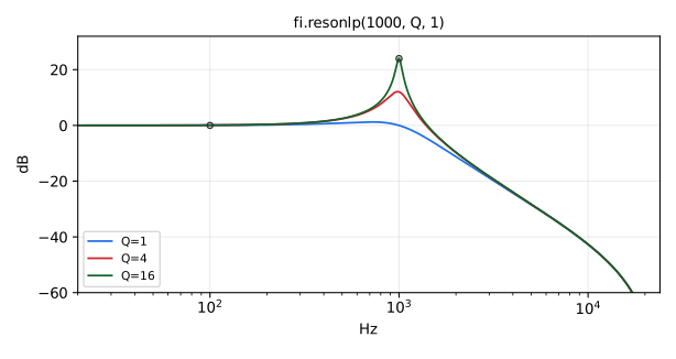
Simple resonant lowpass filter based on tf2s (virtual analog).
resonlp is a standard Faust function.
Usage
_ : resonlp(fc,Q,gain) : _
_ : resonhp(fc,Q,gain) : _
_ : resonbp(fc,Q,gain) : _
Where:
fc: center frequency (Hz)Q: qgain: gain (0-1)
Test
fi = library("filters.lib");
os = library("oscillators.lib");
ba = library("basics.lib");
no = library("noises.lib");
ma = library("maths.lib");
src = os.tosc(440);
resonlp_test = src : fi.resonlp(1000, 2, 0.8);
resonlp_slider_test = no.noise : fi.resonlp(hslider("fc", 1000, 20, 20000, 1), hslider("Q", 2, 0.5, 20, 0.01), hslider("gain", 0.8, 0, 1, 0.01));
resonlp_modulated_test = no.noise : fi.resonlp(20*pow(250, tri), 2, 0.8) with { P = int(ma.SR/10); tri = 1 - abs(2*ba.period(P)/P - 1); };
resonlp_jump_test = no.noise : fi.resonlp(20*pow(250, sq), 2, 0.8) with { P = int(ma.SR/10); sq = ba.period(2*P) < P; };
resonlp_audio_modulated_test = 0.1*no.noise : fi.resonlp(max(20, 1000*(1 + 0.9*os.tosc(500))), 10, 1);
(fi.)resonhp
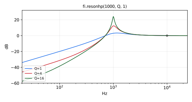
Simple resonant highpass filters based on tf2s (virtual analog).
resonhp is a standard Faust function. It is the second-order highpass
gains^2/(s^2 + s/Q + 1), with s normalized by 2PI*fc: it rolls off at
12 dB per octave below fc, and its gain is gain well above fc.
Usage
_ : resonlp(fc,Q,gain) : _
_ : resonhp(fc,Q,gain) : _
_ : resonbp(fc,Q,gain) : _
Where:
fc: center frequency (Hz)Q: qgain: gain (0-1)
Test
fi = library("filters.lib");
os = library("oscillators.lib");
ba = library("basics.lib");
no = library("noises.lib");
ma = library("maths.lib");
src = os.tosc(440);
resonhp_test = fi.resonhp(1000, 2, 0.8, src);
resonhp_slider_test = no.noise : fi.resonhp(hslider("fc", 1000, 20, 20000, 1), hslider("Q", 2, 0.5, 20, 0.01), hslider("gain", 0.8, 0, 1, 0.01));
resonhp_modulated_test = no.noise : fi.resonhp(20*pow(250, tri), 2, 0.8) with { P = int(ma.SR/10); tri = 1 - abs(2*ba.period(P)/P - 1); };
resonhp_jump_test = no.noise : fi.resonhp(20*pow(250, sq), 2, 0.8) with { P = int(ma.SR/10); sq = ba.period(2*P) < P; };
resonhp_audio_modulated_test = 0.1*no.noise : fi.resonhp(max(20, 1000*(1 + 0.9*os.tosc(500))), 10, 1);
(fi.)resonbp
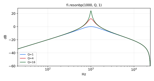
Simple resonant bandpass filters based on tf2s (virtual analog).
resonbp is a standard Faust function. It is
gains/(s^2 + s/Q + 1), with s normalized by 2PIfc, so its peak gain,
at fc, is gainQ.
Usage
_ : resonlp(fc,Q,gain) : _
_ : resonhp(fc,Q,gain) : _
_ : resonbp(fc,Q,gain) : _
Where:
fc: center frequency (Hz)Q: qgain: gain (0-1)
Test
fi = library("filters.lib");
os = library("oscillators.lib");
ba = library("basics.lib");
no = library("noises.lib");
ma = library("maths.lib");
src = os.tosc(440);
resonbp_test = src : fi.resonbp(1000, 2, 0.8);
resonbp_slider_test = no.noise : fi.resonbp(hslider("fc", 1000, 20, 20000, 1), hslider("Q", 2, 0.5, 20, 0.01), hslider("gain", 0.8, 0, 1, 0.01));
resonbp_modulated_test = no.noise : fi.resonbp(20*pow(250, tri), 2, 0.8) with { P = int(ma.SR/10); tri = 1 - abs(2*ba.period(P)/P - 1); };
resonbp_jump_test = no.noise : fi.resonbp(20*pow(250, sq), 2, 0.8) with { P = int(ma.SR/10); sq = ba.period(2*P) < P; };
resonbp_audio_modulated_test = 0.1*no.noise : fi.resonbp(max(20, 1000*(1 + 0.9*os.tosc(500))), 10, 1);
Butterworth Lowpass/Highpass Filters
(fi.)lowpass
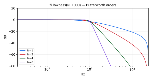
Nth-order Butterworth lowpass filter.
lowpass is a standard Faust function.
Usage
_ : lowpass(N,fc) : _
Where:
N: filter order (number of poles), nonnegative constant numerical expressionfc: desired cut-off frequency (-3dB frequency) in Hz, clamped to [0, 0.499*SR]: 0 holds the filter's states (see the section Digital Filter Sections Specified as Analog Filter Sections)
Test
fi = library("filters.lib");
os = library("oscillators.lib");
no = library("noises.lib");
ba = library("basics.lib");
ma = library("maths.lib");
src = os.tosc(440);
lowpass_test = src : fi.lowpass(4, 2000);
lowpass_lowfc_test = no.noise : fi.lowpass(3, 10.1);
lowpass_zero_freq_test = no.noise : fi.lowpass(3, 1000*max(0, 1 - ba.time/12000) + 1000*(ba.time >= 24000));
lowpass_slider_test = no.noise : fi.lowpass(4, hslider("fc", 2000, 20, 20000, 1));
lowpass_modulated_test = no.noise : fi.lowpass(4, 20*pow(250, tri)) with { P = int(ma.SR/10); tri = 1 - abs(2*ba.period(P)/P - 1); };
lowpass_jump_test = no.noise : fi.lowpass(4, 20*pow(250, sq)) with { P = int(ma.SR/10); sq = ba.period(2*P) < P; };
lowpass_audio_modulated_test = 0.1*no.noise : fi.lowpass(3, max(20, 1000*(1 + 0.9*os.tosc(500))));
References
- https://ccrma.stanford.edu/~jos/filters/Butterworth_Lowpass_Design.html
butterfunction in Octave("[z,p,g] = butter(N,1,'s');")
(fi.)highpass
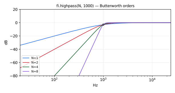
Nth-order Butterworth highpass filter.
highpass is a standard Faust function.
Usage
_ : highpass(N,fc) : _
Where:
N: filter order (number of poles), nonnegative constant numerical expressionfc: desired cut-off frequency (-3dB frequency) in Hz, clamped to [0, 0.499*SR]: 0 holds the filter's states, so that the input passes minus the DC they hold (see the section Digital Filter Sections Specified as Analog Filter Sections)
Test
fi = library("filters.lib");
os = library("oscillators.lib");
no = library("noises.lib");
ba = library("basics.lib");
ma = library("maths.lib");
src = os.tosc(440);
highpass_test = src : fi.highpass(4, 500);
highpass_lowfc_test = no.noise : fi.highpass(3, 10.1);
highpass_zero_freq_test = no.noise : fi.highpass(3, 1000*max(0, 1 - ba.time/12000) + 1000*(ba.time >= 24000));
highpass_slider_test = no.noise : fi.highpass(4, hslider("fc", 500, 20, 20000, 1));
highpass_modulated_test = no.noise : fi.highpass(4, 20*pow(250, tri)) with { P = int(ma.SR/10); tri = 1 - abs(2*ba.period(P)/P - 1); };
highpass_jump_test = no.noise : fi.highpass(4, 20*pow(250, sq)) with { P = int(ma.SR/10); sq = ba.period(2*P) < P; };
highpass_audio_modulated_test = 0.1*no.noise : fi.highpass(3, max(20, 1000*(1 + 0.9*os.tosc(500))));
References
- https://ccrma.stanford.edu/~jos/filters/Butterworth_Lowpass_Design.html
butterfunction in Octave("[z,p,g] = butter(N,1,'s');")
(fi.)lowpass0_highpass1
Generic Butterworth lowpass/highpass filter: the shared implementation
behind fi.lowpass and fi.highpass, with a selector choosing between
the two responses.
Usage
_ : lowpass0_highpass1(s,N,fc) : _
Where:
s: response selector: 0 for lowpass, 1 for highpass (a constant numerical expression)N: filter order (a constant numerical expression)fc: -3dB cutoff frequency in Hz
Method
A first-order section tf1s for odd N, then second-order sections with
the Butterworth pole angles. Each second-order section has the transfer
function of tf2s (bilinear transform prewarped at fc), computed in
trapezoidal state-variable form (svf.lp/svf.hp), which stays accurate in
single precision when fc is small relative to the sample rate.
Test
fi = library("filters.lib");
os = library("oscillators.lib");
ba = library("basics.lib");
no = library("noises.lib");
ma = library("maths.lib");
src = os.tosc(440);
lowpass0_highpass1_test = src : fi.lowpass0_highpass1(0, 2, 1000);
lowpass0_highpass1_slider_test = no.noise : fi.lowpass0_highpass1(0, 2, hslider("fc", 1000, 20, 20000, 1));
lowpass0_highpass1_modulated_test = no.noise : fi.lowpass0_highpass1(0, 2, 20*pow(250, tri)) with { P = int(ma.SR/10); tri = 1 - abs(2*ba.period(P)/P - 1); };
lowpass0_highpass1_jump_test = no.noise : fi.lowpass0_highpass1(0, 2, 20*pow(250, sq)) with { P = int(ma.SR/10); sq = ba.period(2*P) < P; };
(fi.)lowpass_tpt_df, (fi.)highpass_tpt_df
lowpass and highpass (order-N Butterworth) in trapezoidal sections
below the cutoff limit L and in direct-form sections (tf2s_df,
tf1s_df) at and above it. With a constant fc, only one of the two is
compiled. With a varying fc, both run (more CPU than either), the
direct form at max(fc, L) so that it stays accurate, and the output
switches between them where fc crosses L: pass L = ma.MAX
(trapezoidal) or L = 0 (direct form) to compile one form only.
Usage
_ : lowpass_tpt_df(L,N,fc) : _
_ : highpass_tpt_df(L,N,fc) : _
Where:
L: cutoff limit in Hz, usuallytpt_df_fmin;L <= 0selects the direct form andL >= ma.MAXthe trapezoidal form for everyfcN: filter order (number of poles), a constant numerical expressionfc: cutoff frequency in Hz
Test
fi = library("filters.lib");
no = library("noises.lib");
ba = library("basics.lib");
ma = library("maths.lib");
lowpass_tpt_df_test = no.noise : fi.lowpass_tpt_df(fi.tpt_df_fmin, 5, 4000);
lowpass_tpt_df_low_test = no.noise : fi.lowpass_tpt_df(fi.tpt_df_fmin, 5, 50);
lowpass_tpt_df_slider_test = no.noise : fi.lowpass_tpt_df(fi.tpt_df_fmin, 3, hslider("fc", 1000, 20, 20000, 1));
lowpass_tpt_df_modulated_test = no.noise : fi.lowpass_tpt_df(0, 3, 2500*pow(8, tri)) with { P = int(ma.SR/10); tri = 1 - abs(2*ba.period(P)/P - 1); };
lowpass_tpt_df_jump_test = no.noise : fi.lowpass_tpt_df(ma.MAX, 3, 20*pow(250, sq)) with { P = int(ma.SR/10); sq = ba.period(2*P) < P; };
highpass_tpt_df_test = no.noise : fi.highpass_tpt_df(fi.tpt_df_fmin, 5, 4000);
highpass_tpt_df_low_test = no.noise : fi.highpass_tpt_df(fi.tpt_df_fmin, 5, 50);
highpass_tpt_df_slider_test = no.noise : fi.highpass_tpt_df(fi.tpt_df_fmin, 3, hslider("fc", 1000, 20, 20000, 1));
highpass_tpt_df_modulated_test = no.noise : fi.highpass_tpt_df(0, 3, 2500*pow(8, tri)) with { P = int(ma.SR/10); tri = 1 - abs(2*ba.period(P)/P - 1); };
highpass_tpt_df_jump_test = no.noise : fi.highpass_tpt_df(ma.MAX, 3, 20*pow(250, sq)) with { P = int(ma.SR/10); sq = ba.period(2*P) < P; };
Special Filter-Bank Delay-Equalizing Allpass Filters
These special allpass filters are needed by filterbank et al. below.
They are equivalent to highpass(N,fc) +|- lowpass(N,fc), but with
canceling pole-zero pairs removed (which occurs for odd N). Both the sum
and the difference are allpass for odd N only, the order the filter banks
require.
(fi.)highpass_plus_lowpass
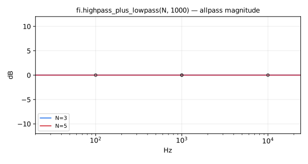
Sum of the order-N Butterworth highpass and lowpass responses at the same
cutoff: for odd N, an allpass used as delay equalizer by fi.filterbank
and the filter banks below. For odd orders 1, 3 and 5, canceling pole-zero
pairs are removed. For even N the sum is not allpass: it has a notch at
fc for N=2, and +3 dB at fc for N=4.
Usage
_ : highpass_plus_lowpass(N,fc) : _
Where:
N: filter order (a constant numerical expression)fc: crossover frequency in Hz
Test
fi = library("filters.lib");
os = library("oscillators.lib");
ba = library("basics.lib");
no = library("noises.lib");
ma = library("maths.lib");
highpass_plus_lowpass_test = os.tosc(440) : fi.highpass_plus_lowpass(3, 1000);
highpass_plus_lowpass_slider_test = no.noise : fi.highpass_plus_lowpass(3, hslider("fc", 1000, 20, 20000, 1));
highpass_plus_lowpass_modulated_test = no.noise : fi.highpass_plus_lowpass(3, 20*pow(250, tri)) with { P = int(ma.SR/10); tri = 1 - abs(2*ba.period(P)/P - 1); };
highpass_plus_lowpass_jump_test = no.noise : fi.highpass_plus_lowpass(3, 20*pow(250, sq)) with { P = int(ma.SR/10); sq = ba.period(2*P) < P; };
(fi.)highpass_minus_lowpass
Difference between the order-N Butterworth highpass and lowpass responses
at the same cutoff: an allpass used as delay equalizer by the
dc-inverted filter banks (fi.mth_octave_filterbank_alt). For odd orders
3 and 5, canceling pole-zero pairs are removed.
Usage
_ : highpass_minus_lowpass(N,fc) : _
Where:
N: filter order (a constant numerical expression)fc: crossover frequency in Hz
Test
fi = library("filters.lib");
os = library("oscillators.lib");
ba = library("basics.lib");
no = library("noises.lib");
ma = library("maths.lib");
highpass_minus_lowpass_test = os.tosc(440) : fi.highpass_minus_lowpass(3, 1000);
highpass_minus_lowpass_slider_test = no.noise : fi.highpass_minus_lowpass(3, hslider("fc", 1000, 20, 20000, 1));
highpass_minus_lowpass_modulated_test = no.noise : fi.highpass_minus_lowpass(3, 20*pow(250, tri)) with { P = int(ma.SR/10); tri = 1 - abs(2*ba.period(P)/P - 1); };
highpass_minus_lowpass_jump_test = no.noise : fi.highpass_minus_lowpass(3, 20*pow(250, sq)) with { P = int(ma.SR/10); sq = ba.period(2*P) < P; };
(fi.)highpass_plus_lowpass_tpt_df, (fi.)highpass_minus_lowpass_tpt_df
highpass_plus_lowpass and highpass_minus_lowpass in trapezoidal
sections below the cutoff limit L and in direct-form sections
(tf2s_df, tf1s_df) at and above it, as in lowpass_tpt_df: the delay
equalizers of the *_tpt_df filter banks.
Usage
_ : highpass_plus_lowpass_tpt_df(L,N,fc) : _
_ : highpass_minus_lowpass_tpt_df(L,N,fc) : _
Where:
L: cutoff limit in Hz, usuallytpt_df_fmin;L <= 0selects the direct form andL >= ma.MAXthe trapezoidal form for everyfcN: filter order (a constant numerical expression)fc: crossover frequency in Hz
Test
fi = library("filters.lib");
no = library("noises.lib");
ba = library("basics.lib");
ma = library("maths.lib");
highpass_plus_lowpass_tpt_df_test = no.noise : fi.highpass_plus_lowpass_tpt_df(fi.tpt_df_fmin, 5, 4000);
highpass_plus_lowpass_tpt_df_low_test = no.noise : fi.highpass_plus_lowpass_tpt_df(fi.tpt_df_fmin, 3, 50);
highpass_plus_lowpass_tpt_df_slider_test = no.noise : fi.highpass_plus_lowpass_tpt_df(fi.tpt_df_fmin, 5, hslider("fc", 1000, 20, 20000, 1));
highpass_plus_lowpass_tpt_df_modulated_test = no.noise : fi.highpass_plus_lowpass_tpt_df(0, 5, 2500*pow(8, tri)) with { P = int(ma.SR/10); tri = 1 - abs(2*ba.period(P)/P - 1); };
highpass_plus_lowpass_tpt_df_jump_test = no.noise : fi.highpass_plus_lowpass_tpt_df(ma.MAX, 5, 20*pow(250, sq)) with { P = int(ma.SR/10); sq = ba.period(2*P) < P; };
highpass_minus_lowpass_tpt_df_test = no.noise : fi.highpass_minus_lowpass_tpt_df(fi.tpt_df_fmin, 5, 4000);
highpass_minus_lowpass_tpt_df_low_test = no.noise : fi.highpass_minus_lowpass_tpt_df(fi.tpt_df_fmin, 3, 50);
highpass_minus_lowpass_tpt_df_slider_test = no.noise : fi.highpass_minus_lowpass_tpt_df(fi.tpt_df_fmin, 5, hslider("fc", 1000, 20, 20000, 1));
highpass_minus_lowpass_tpt_df_modulated_test = no.noise : fi.highpass_minus_lowpass_tpt_df(0, 5, 2500*pow(8, tri)) with { P = int(ma.SR/10); tri = 1 - abs(2*ba.period(P)/P - 1); };
highpass_minus_lowpass_tpt_df_jump_test = no.noise : fi.highpass_minus_lowpass_tpt_df(ma.MAX, 5, 20*pow(250, sq)) with { P = int(ma.SR/10); sq = ba.period(2*P) < P; };
(fi.)highpass_plus_lowpass_even
Sum of the even-order Butterworth highpass and lowpass responses,
highpass(N,fc) + lowpass(N,fc). Takes two copies of the input signal
(both normally fed the same signal); fi.highpass_plus_lowpass selects
this case automatically for even N.
Usage
_,_ : highpass_plus_lowpass_even(N,fc) : _
Where:
N: even filter order (a constant numerical expression)fc: crossover frequency in Hz
Test
fi = library("filters.lib");
os = library("oscillators.lib");
ba = library("basics.lib");
no = library("noises.lib");
ma = library("maths.lib");
highpass_plus_lowpass_even_test = os.tosc(440), os.tosc(440) : fi.highpass_plus_lowpass_even(4, 1000);
highpass_plus_lowpass_even_slider_test = (no.noise <: _, _) : fi.highpass_plus_lowpass_even(4, hslider("fc", 1000, 20, 20000, 1));
highpass_plus_lowpass_even_modulated_test = (no.noise <: _, _) : fi.highpass_plus_lowpass_even(4, 20*pow(250, tri)) with { P = int(ma.SR/10); tri = 1 - abs(2*ba.period(P)/P - 1); };
highpass_plus_lowpass_even_jump_test = (no.noise <: _, _) : fi.highpass_plus_lowpass_even(4, 20*pow(250, sq)) with { P = int(ma.SR/10); sq = ba.period(2*P) < P; };
(fi.)highpass_minus_lowpass_even
Difference between the even-order Butterworth highpass and lowpass
responses, highpass(N,fc) - lowpass(N,fc). Takes two copies of the input
signal (both normally fed the same signal); fi.highpass_minus_lowpass
selects this case automatically for even N.
Usage
_,_ : highpass_minus_lowpass_even(N,fc) : _
Where:
N: even filter order (a constant numerical expression)fc: crossover frequency in Hz
Test
fi = library("filters.lib");
os = library("oscillators.lib");
ba = library("basics.lib");
no = library("noises.lib");
ma = library("maths.lib");
highpass_minus_lowpass_even_test = os.tosc(440), os.tosc(440) : fi.highpass_minus_lowpass_even(4, 1000);
highpass_minus_lowpass_even_slider_test = (no.noise <: _, _) : fi.highpass_minus_lowpass_even(4, hslider("fc", 1000, 20, 20000, 1));
highpass_minus_lowpass_even_modulated_test = (no.noise <: _, _) : fi.highpass_minus_lowpass_even(4, 20*pow(250, tri)) with { P = int(ma.SR/10); tri = 1 - abs(2*ba.period(P)/P - 1); };
highpass_minus_lowpass_even_jump_test = (no.noise <: _, _) : fi.highpass_minus_lowpass_even(4, 20*pow(250, sq)) with { P = int(ma.SR/10); sq = ba.period(2*P) < P; };
(fi.)highpass_plus_lowpass_odd
Sum of the odd-order highpass and lowpass responses.
Usage
_,_ : highpass_plus_lowpass_odd(N,fc) : _
Where:
N: odd Butterworth orderfc: cutoff frequency in Hz
Test
fi = library("filters.lib");
os = library("oscillators.lib");
ba = library("basics.lib");
no = library("noises.lib");
ma = library("maths.lib");
highpass_plus_lowpass_odd_test = os.tosc(440), os.tosc(440) : fi.highpass_plus_lowpass_odd(3, 1000);
highpass_plus_lowpass_odd_slider_test = (no.noise <: _, _) : fi.highpass_plus_lowpass_odd(3, hslider("fc", 1000, 20, 20000, 1));
highpass_plus_lowpass_odd_modulated_test = (no.noise <: _, _) : fi.highpass_plus_lowpass_odd(3, 20*pow(250, tri)) with { P = int(ma.SR/10); tri = 1 - abs(2*ba.period(P)/P - 1); };
highpass_plus_lowpass_odd_jump_test = (no.noise <: _, _) : fi.highpass_plus_lowpass_odd(3, 20*pow(250, sq)) with { P = int(ma.SR/10); sq = ba.period(2*P) < P; };
FIXME: Rewrite the following, as for orders 3 and 5 above, to eliminate pole-zero cancellations:
(fi.)highpass_minus_lowpass_odd
Difference between the odd-order highpass and lowpass responses.
Usage
_,_ : highpass_minus_lowpass_odd(N,fc) : _
Where:
N: odd Butterworth orderfc: cutoff frequency in Hz
Test
fi = library("filters.lib");
os = library("oscillators.lib");
ba = library("basics.lib");
no = library("noises.lib");
ma = library("maths.lib");
highpass_minus_lowpass_odd_test = os.tosc(440), os.tosc(440) : fi.highpass_minus_lowpass_odd(3, 1000);
highpass_minus_lowpass_odd_slider_test = (no.noise <: _, _) : fi.highpass_minus_lowpass_odd(3, hslider("fc", 1000, 20, 20000, 1));
highpass_minus_lowpass_odd_modulated_test = (no.noise <: _, _) : fi.highpass_minus_lowpass_odd(3, 20*pow(250, tri)) with { P = int(ma.SR/10); tri = 1 - abs(2*ba.period(P)/P - 1); };
highpass_minus_lowpass_odd_jump_test = (no.noise <: _, _) : fi.highpass_minus_lowpass_odd(3, 20*pow(250, sq)) with { P = int(ma.SR/10); sq = ba.period(2*P) < P; };
FIXME: Rewrite the following, as for orders 3 and 5 above, to eliminate pole-zero cancellations/
Elliptic (Cauer) Lowpass Filters
Elliptic (Cauer) Lowpass Filters
References
- http://en.wikipedia.org/wiki/Elliptic_filter
- functions
ncauerandellipin Octave.
(fi.)lowpass3e
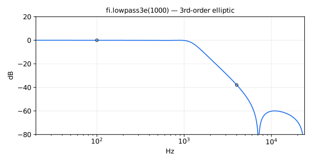
Third-order Elliptic (Cauer) lowpass filter.
Usage
_ : lowpass3e(fc) : _
Where:
fc: passband edge frequency in Hz, where the gain is -0.2 dB (the -3 dB point is near 1.28*fc)
Test
fi = library("filters.lib");
os = library("oscillators.lib");
ba = library("basics.lib");
no = library("noises.lib");
src = os.tosc(440);
lowpass3e_test = src : fi.lowpass3e(1000);
lowpass3e_slider_test = no.noise : fi.lowpass3e(hslider("fc", 1000, 20, 20000, 1));
Design
For spectral band-slice level display (see octave_analyzer3e):
[z,p,g] = ncauer(Rp,Rs,3);  % analog zeros, poles, and gain, where
Rp = 60  % dB ripple in stopband
Rs = 0.2 % dB ripple in passband
(fi.)lowpass6e
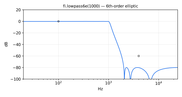
Sixth-order Elliptic/Cauer lowpass filter.
Usage
_ : lowpass6e(fc) : _
Where:
fc: passband edge frequency in Hz, where the gain is -0.2 dB (the -3 dB point is near 1.06*fc)
Test
fi = library("filters.lib");
os = library("oscillators.lib");
no = library("noises.lib");
src = os.tosc(440);
lowpass6e_test = src : fi.lowpass6e(1000);
lowpass6e_slider_test = no.noise : fi.lowpass6e(hslider("fc", 1000, 20, 20000, 1));
Design
For spectral band-slice level display (see octave_analyzer6e):
[z,p,g] = ncauer(Rp,Rs,6);  % analog zeros, poles, and gain, where
 Rp = 80  % dB ripple in stopband
 Rs = 0.2 % dB ripple in passband
Elliptic Highpass Filters
(fi.)highpass3e
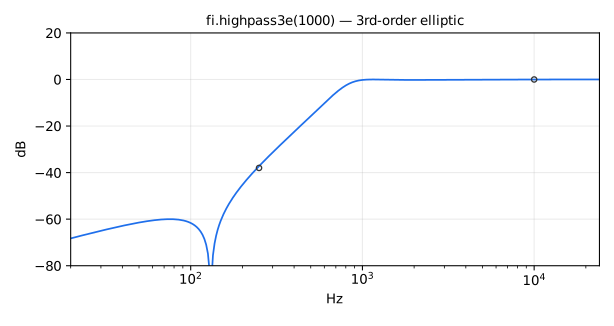
Third-order Elliptic (Cauer) highpass filter. Inversion of lowpass3e wrt unit
circle in s plane (s <- 1/s).
Usage
_ : highpass3e(fc) : _
Where:
fc: passband edge frequency in Hz, where the gain is -0.2 dB (the -3 dB point is near fc/1.28)
Test
fi = library("filters.lib");
os = library("oscillators.lib");
ba = library("basics.lib");
no = library("noises.lib");
ma = library("maths.lib");
src = os.tosc(440);
highpass3e_test = src : fi.highpass3e(1000);
highpass3e_slider_test = no.noise : fi.highpass3e(hslider("fc", 1000, 20, 20000, 1));
highpass3e_modulated_test = no.noise : fi.highpass3e(20*pow(250, tri)) with { P = int(ma.SR/10); tri = 1 - abs(2*ba.period(P)/P - 1); };
highpass3e_jump_test = no.noise : fi.highpass3e(20*pow(250, sq)) with { P = int(ma.SR/10); sq = ba.period(2*P) < P; };
(fi.)highpass6e
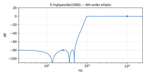
Sixth-order Elliptic/Cauer highpass filter. Inversion of lowpass6e wrt unit
circle in s plane (s <- 1/s).
Usage
_ : highpass6e(fc) : _
Where:
fc: passband edge frequency in Hz, where the gain is -0.2 dB (the -3 dB point is near fc/1.06)
Test
fi = library("filters.lib");
os = library("oscillators.lib");
ba = library("basics.lib");
no = library("noises.lib");
ma = library("maths.lib");
src = os.tosc(440);
highpass6e_test = src : fi.highpass6e(1000);
highpass6e_slider_test = no.noise : fi.highpass6e(hslider("fc", 1000, 20, 20000, 1));
highpass6e_modulated_test = no.noise : fi.highpass6e(20*pow(250, tri)) with { P = int(ma.SR/10); tri = 1 - abs(2*ba.period(P)/P - 1); };
highpass6e_jump_test = no.noise : fi.highpass6e(20*pow(250, sq)) with { P = int(ma.SR/10); sq = ba.period(2*P) < P; };
(fi.)lowpass6e_tpt_df, (fi.)highpass6e_tpt_df
lowpass6e and highpass6e in trapezoidal sections below the cutoff
limit L and in direct-form sections (tf2s_df) at and above it, as in
lowpass_tpt_df: the band splits of an.mth_octave_analyzer6e_tpt_df.
Usage
_ : lowpass6e_tpt_df(L,fc) : _
_ : highpass6e_tpt_df(L,fc) : _
Where:
L: cutoff limit in Hz, usuallytpt_df_fmin;L <= 0selects the direct form andL >= ma.MAXthe trapezoidal form for everyfcfc: -3dB frequency in Hz
Test
fi = library("filters.lib");
no = library("noises.lib");
ba = library("basics.lib");
ma = library("maths.lib");
lowpass6e_tpt_df_test = no.noise : fi.lowpass6e_tpt_df(fi.tpt_df_fmin, 4000);
lowpass6e_tpt_df_low_test = no.noise : fi.lowpass6e_tpt_df(fi.tpt_df_fmin, 50);
lowpass6e_tpt_df_slider_test = no.noise : fi.lowpass6e_tpt_df(fi.tpt_df_fmin, hslider("fc", 1000, 20, 20000, 1));
lowpass6e_tpt_df_modulated_test = no.noise : fi.lowpass6e_tpt_df(0, 2500*pow(8, tri)) with { P = int(ma.SR/10); tri = 1 - abs(2*ba.period(P)/P - 1); };
lowpass6e_tpt_df_jump_test = no.noise : fi.lowpass6e_tpt_df(ma.MAX, 20*pow(250, sq)) with { P = int(ma.SR/10); sq = ba.period(2*P) < P; };
highpass6e_tpt_df_test = no.noise : fi.highpass6e_tpt_df(fi.tpt_df_fmin, 4000);
highpass6e_tpt_df_low_test = no.noise : fi.highpass6e_tpt_df(fi.tpt_df_fmin, 50);
highpass6e_tpt_df_slider_test = no.noise : fi.highpass6e_tpt_df(fi.tpt_df_fmin, hslider("fc", 1000, 20, 20000, 1));
highpass6e_tpt_df_modulated_test = no.noise : fi.highpass6e_tpt_df(0, 2500*pow(8, tri)) with { P = int(ma.SR/10); tri = 1 - abs(2*ba.period(P)/P - 1); };
highpass6e_tpt_df_jump_test = no.noise : fi.highpass6e_tpt_df(ma.MAX, 20*pow(250, sq)) with { P = int(ma.SR/10); sq = ba.period(2*P) < P; };
Butterworth Bandpass/Bandstop Filters
(fi.)bandpass
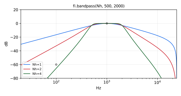
Order 2*Nh Butterworth bandpass filter made using the transformation
s <- s + wc^2/s on lowpass(Nh), where wc is the desired bandpass center
frequency. The lowpass(Nh) cutoff w1 is the desired bandpass width.
bandpass is a standard Faust function.
Usage
_ : bandpass(Nh,fl,fu) : _
Where:
Nh: HALF the desired bandpass order (which is therefore even)fl: lower -3dB frequency in Hzfu: upper -3dB frequency in Hz Thus, the passband width isfu-fl, and its center frequency, where the response peaks, is the geometric mean of the band edges prewarped by the bilinear transform:sqrt(fl*fu)well below Nyquist, somewhat higher near it.fuis clamped to [0, 0.499*SR] andflto [0,fu]:fl= 0 giveslowpass(Nh, fu), andflcan be swept to 0 or jump to and from it without a click or a spike (seetf2sb). The passband width is floored at 5e-4 times the center frequency (a Q of at most 2000), sofl=fugives that narrowest band, and a band can close and reopen without a spike.
Test
fi = library("filters.lib");
os = library("oscillators.lib");
no = library("noises.lib");
ba = library("basics.lib");
ma = library("maths.lib");
src = os.tosc(440);
bandpass_test = src : fi.bandpass(2, 500, 1500);
bandpass_lowband_test = no.noise : fi.bandpass(2, 100, 200);
bandpass_narrowlow_test = no.noise : fi.bandpass(2, 20, 22);
bandpass_zero_freq_test = no.noise : fi.bandpass(2, 1000*max(0, 1 - ba.time/12000) + 1000*(ba.time >= 24000), 2000);
bandpass3_zero_freq_test = no.noise : fi.bandpass(3, 1000*max(0, 1 - ba.time/12000) + 1000*(ba.time >= 24000), 2000);
bandpass_nyquist_test = no.noise : fi.bandpass(2, 1000, 0.6*ma.SR);
bandpass_zero_width_test = no.noise : fi.bandpass(2, select2(z, 707.1, 1000), select2(z, 1414.2, 1000)) with { z = (ba.time >= 4800) & (ba.time < 9600); };
bandpass3_zero_width_test = no.noise : fi.bandpass(3, select2(z, 707.1, 1000), select2(z, 1414.2, 1000)) with { z = (ba.time >= 4800) & (ba.time < 9600); };
bandpass_slider_test = no.noise : fi.bandpass(2, hslider("fl", 500, 20, 20000, 1), hslider("fu", 1500, 20, 20000, 1));
bandpass_modulated_test = no.noise : fi.bandpass(2, fl, 3*fl) with { P = int(ma.SR/10); tri = 1 - abs(2*ba.period(P)/P - 1); fl = 20*pow(250, tri); };
bandpass_jump_test = no.noise : fi.bandpass(2, fl, 3*fl) with { P = int(ma.SR/10); sq = ba.period(2*P) < P; fl = 20*pow(250, sq); };
(fi.)bandstop
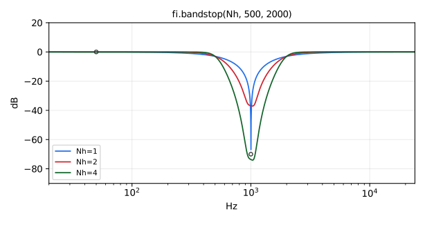
Order 2*Nh Butterworth bandstop filter made using the transformation
s <- s + wc^2/s on highpass(Nh), where wc is the desired bandpass center
frequency. The highpass(Nh) cutoff w1 is the desired bandstop width.
bandstop is a standard Faust function.
Usage
_ : bandstop(Nh,fl,fu) : _
Where:
Nh: HALF the desired bandstop order (which is therefore even)fl: lower -3dB frequency in Hzfu: upper -3dB frequency in Hz Thus, the stopband width isfu-fl, and its center frequency, where the response has its zero, is the geometric mean of the band edges prewarped by the bilinear transform:sqrt(fl*fu)well below Nyquist, somewhat higher near it.fuis clamped to [0, 0.499*SR] andflto [0,fu]:fl= 0 giveshighpass(Nh, fu), andflcan be swept to 0 or jump to and from it without a click or a spike (seetf2sb);fl=fugives the narrowest stopband: the width is floored at 5e-4 times the center frequency, as inbandpass.
Test
fi = library("filters.lib");
os = library("oscillators.lib");
no = library("noises.lib");
ba = library("basics.lib");
ma = library("maths.lib");
src = os.tosc(440);
bandstop_test = src : fi.bandstop(2, 500, 1500);
bandstop_wide_test = no.noise : fi.bandstop(2, 5000, 8000);
bandstop_zero_freq_test = no.noise : fi.bandstop(2, 1000*max(0, 1 - ba.time/12000) + 1000*(ba.time >= 24000), 2000);
bandstop_zero_width_test = no.noise : fi.bandstop(2, select2(z, 707.1, 1000), select2(z, 1414.2, 1000)) with { z = (ba.time >= 4800) & (ba.time < 9600); };
bandstop_slider_test = no.noise : fi.bandstop(2, hslider("fl", 500, 20, 20000, 1), hslider("fu", 1500, 20, 20000, 1));
bandstop_modulated_test = no.noise : fi.bandstop(2, fl, 3*fl) with { P = int(ma.SR/10); tri = 1 - abs(2*ba.period(P)/P - 1); fl = 20*pow(250, tri); };
bandstop_jump_test = no.noise : fi.bandstop(2, fl, 3*fl) with { P = int(ma.SR/10); sq = ba.period(2*P) < P; fl = 20*pow(250, sq); };
(fi.)bandpass0_bandstop1
Generic Butterworth bandpass/bandstop filter: the shared implementation
behind fi.bandpass and fi.bandstop, with a selector choosing between
the two responses.
Usage
_ : bandpass0_bandstop1(s,Nh,fl,fu) : _
Where:
s: response selector: 0 for bandpass, 1 for bandstop (a constant numerical expression)Nh: HALF the filter order, i.e. the number of second-order sections (a constant numerical expression)fl: lower -3dB band edge frequency in Hzfu: upper -3dB band edge frequency in Hz
Test
fi = library("filters.lib");
os = library("oscillators.lib");
ba = library("basics.lib");
no = library("noises.lib");
ma = library("maths.lib");
src = os.tosc(440);
bandpass0_bandstop1_test = src : fi.bandpass0_bandstop1(0, 2, 500, 1500);
bandpass0_bandstop1_slider_test = no.noise : fi.bandpass0_bandstop1(0, 2, hslider("fl", 500, 20, 20000, 1), hslider("fu", 1500, 20, 20000, 1));
bandpass0_bandstop1_modulated_test = no.noise : fi.bandpass0_bandstop1(0, 2, fl, 3*fl) with { P = int(ma.SR/10); tri = 1 - abs(2*ba.period(P)/P - 1); fl = 20*pow(250, tri); };
bandpass0_bandstop1_jump_test = no.noise : fi.bandpass0_bandstop1(0, 2, fl, 3*fl) with { P = int(ma.SR/10); sq = ba.period(2*P) < P; fl = 20*pow(250, sq); };
Elliptic Bandpass Filters
(fi.)bandpass6e
Order 6 elliptic bandpass filter analogous to bandpass(3): a third-order
elliptic lowpass prototype mapped to a bandpass, with a 0.2 dB equiripple
passband between fl and fu.
Usage
_ : bandpass6e(fl,fu) : _
Where:
fl: lower passband edge frequency in Hz (-0.2 dB), clamped to [0,fu] (0 gives the elliptic lowpass atfu; the width is floored at 5e-4 times the center frequency; seebandpass)fu: upper passband edge frequency in Hz (-0.2 dB), clamped to [0, 0.499*SR]
Test
fi = library("filters.lib");
os = library("oscillators.lib");
ba = library("basics.lib");
no = library("noises.lib");
ma = library("maths.lib");
src = os.tosc(440);
bandpass6e_test = src : fi.bandpass6e(500, 1500);
bandpass6e_zero_freq_test = no.noise : fi.bandpass6e(1000*max(0, 1 - ba.time/12000) + 1000*(ba.time >= 24000), 2000);
bandpass6e_slider_test = no.noise : fi.bandpass6e(hslider("fl", 500, 20, 20000, 1), hslider("fu", 1500, 20, 20000, 1));
bandpass6e_modulated_test = no.noise : fi.bandpass6e(fl, 3*fl) with { P = int(ma.SR/10); tri = 1 - abs(2*ba.period(P)/P - 1); fl = 20*pow(250, tri); };
bandpass6e_jump_test = no.noise : fi.bandpass6e(fl, 3*fl) with { P = int(ma.SR/10); sq = ba.period(2*P) < P; fl = 20*pow(250, sq); };
(fi.)bandpass12e
Order 12 elliptic bandpass filter analogous to bandpass(6): a sixth-order
elliptic lowpass prototype mapped to a bandpass, with a 0.2 dB equiripple
passband between fl and fu.
Usage
_ : bandpass12e(fl,fu) : _
Where:
fl: lower passband edge frequency in Hz (-0.2 dB), clamped to [0,fu] (0 gives the elliptic lowpass atfu; the width is floored at 5e-4 times the center frequency; seebandpass)fu: upper passband edge frequency in Hz (-0.2 dB), clamped to [0, 0.499*SR]
Test
fi = library("filters.lib");
os = library("oscillators.lib");
ba = library("basics.lib");
no = library("noises.lib");
ma = library("maths.lib");
src = os.tosc(440);
bandpass12e_test = src : fi.bandpass12e(500, 1500);
bandpass12e_zero_freq_test = no.noise : fi.bandpass12e(1000*max(0, 1 - ba.time/12000) + 1000*(ba.time >= 24000), 2000);
bandpass12e_slider_test = no.noise : fi.bandpass12e(hslider("fl", 500, 20, 20000, 1), hslider("fu", 1500, 20, 20000, 1));
bandpass12e_modulated_test = no.noise : fi.bandpass12e(fl, 3*fl) with { P = int(ma.SR/10); tri = 1 - abs(2*ba.period(P)/P - 1); fl = 20*pow(250, tri); };
bandpass12e_jump_test = no.noise : fi.bandpass12e(fl, 3*fl) with { P = int(ma.SR/10); sq = ba.period(2*P) < P; fl = 20*pow(250, sq); };
(fi.)pospass
Positive-Pass Filter (single-side-band filter).
Usage
_ : pospass(N,fc) : _,_
where
N: filter order (Butterworth bandpass for positive frequencies).fc: lower bandpass cutoff frequency in Hz.- Highpass cutoff frequency at ma.SR/2 - fc Hz.
Example test program
- See
dm.pospass_demo - Look at frequency response
Method
A filter passing only positive frequencies can be made from a half-band lowpass by modulating it up to the positive-frequency range. Equivalently, down-modulate the input signal using a complex sinusoid at -SR/4 Hz, lowpass it with a half-band filter, and modulate back up by SR/4 Hz. In Faust/math notation:
An approximation to the Hilbert transform is given by the imaginary output signal:
hilbert(N) = pospass(N) : !,*(2);
Test
fi = library("filters.lib");
ba = library("basics.lib");
no = library("noises.lib");
os = library("oscillators.lib");
ma = library("maths.lib");
src = os.tosc(440);
pospass_test = src : fi.pospass(3, 1000);
pospass_slider_test = no.noise : fi.pospass(3, hslider("fc", 1000, 20, 20000, 1));
pospass_modulated_test = no.noise : fi.pospass(3, 20*pow(250, tri)) with { P = int(ma.SR/10); tri = 1 - abs(2*ba.period(P)/P - 1); };
pospass_jump_test = no.noise : fi.pospass(3, 20*pow(250, sq)) with { P = int(ma.SR/10); sq = ba.period(2*P) < P; };
References
- https://ccrma.stanford.edu/~jos/mdft/Analytic_Signals_Hilbert_Transform.html
- https://ccrma.stanford.edu/~jos/sasp/Comparison_Optimal_Chebyshev_FIR_I.html
- https://ccrma.stanford.edu/~jos/sasp/Hilbert_Transform.html
(fi.)pospass6e
Positive-pass filter like pospass, but built on the order-6 elliptic
lowpass lowpass6e instead of a Butterworth lowpass: a steeper
transition band for the same order.
Usage
_ : pospass6e(fc) : _,_
Where:
fc: lower cutoff frequency in Hz
Test
fi = library("filters.lib");
os = library("oscillators.lib");
ba = library("basics.lib");
no = library("noises.lib");
ma = library("maths.lib");
pospass6e_test = os.tosc(440) : fi.pospass6e(100);
pospass6e_slider_test = no.noise : fi.pospass6e(hslider("fc", 100, 20, 20000, 1));
pospass6e_modulated_test = no.noise : fi.pospass6e(20*pow(250, tri)) with { P = int(ma.SR/10); tri = 1 - abs(2*ba.period(P)/P - 1); };
pospass6e_jump_test = no.noise : fi.pospass6e(20*pow(250, sq)) with { P = int(ma.SR/10); sq = ba.period(2*P) < P; };
(fi.)hilbert
Approximate Hilbert transform: twice the imaginary part of the analytic
signal computed by fi.pospass, i.e. a signal in quadrature (-90 degrees)
with the in-phase (real) output of the same filter. This is the one-line
construction given in the fi.pospass documentation.
The output carries the group delay of the underlying filter, so pair it
with the real part of fi.pospass (not with the raw input) when phase
alignment matters. Accuracy improves with the order N and with the input
frequency: rejecting the negative-frequency image of a component at f Hz
requires the internal half-band lowpass to cut inside a transition band of
width 2*f, so low frequencies demand high orders (measured at 48 kHz:
with N = 8, a 5 kHz sine yields an analytic pair with 0.5% envelope
ripple and quadrature to 1e-4, while a 1 kHz sine needs N around 32 for
comparable quality).
Usage
_ : hilbert(N,fc) : _
Where:
N: order of the underlying Butterworth positive-pass filter (a constant numerical expression)fc: lower cutoff frequency in Hz of the positive-pass filter
Test
fi = library("filters.lib");
os = library("oscillators.lib");
ba = library("basics.lib");
no = library("noises.lib");
ma = library("maths.lib");
hilbert_test = os.tosc(440) : fi.hilbert(4, 20);
hilbert_slider_test = no.noise : fi.hilbert(4, hslider("fc", 20, 5, 500, 1));
hilbert_modulated_test = no.noise : fi.hilbert(4, 10*pow(10, tri)) with { P = int(ma.SR/10); tri = 1 - abs(2*ba.period(P)/P - 1); };
hilbert_jump_test = no.noise : fi.hilbert(4, 10*pow(10, sq)) with { P = int(ma.SR/10); sq = ba.period(2*P) < P; };
References
- https://ccrma.stanford.edu/~jos/mdft/Analytic_Signals_Hilbert_Transform.html
- https://ccrma.stanford.edu/~jos/sasp/Hilbert_Transform.html
Parametric Equalizers (Shelf, Peaking)
Parametric Equalizers (Shelf, Peaking).
References
- http://en.wikipedia.org/wiki/Equalization
- https://webaudio.github.io/Audio-EQ-Cookbook/Audio-EQ-Cookbook.txt
- Digital Audio Signal Processing, Udo Zolzer, Wiley, 1999, p. 124
- https://ccrma.stanford.edu/~jos/filters/Low_High_Shelving_Filters.html
- https://ccrma.stanford.edu/~jos/filters/Peaking_Equalizers.html
- maxmsp.lib in the Faust distribution
- bandfilter.dsp in the faust2pd distribution
(fi.)lowshelf
Order-N "low shelf" filter (gain boost|cut between dc and some frequency)
low_shelf is a standard Faust function.
Usage
_ : lowshelf(N,L0,fx) : _
_ : low_shelf(L0,fx) : _ // default case (order 3)
_ : lowshelf_other_freq(N,L0,fx) : _
Where:
N: filter order 1, 3, 5, ... (odd only, default should be 3, a constant numerical expression)L0: desired level (dB) between dc and fx (boostL0>0or cutL0<0)fx: -3dB frequency of lowpass band (L0>0) or upper band (L0<0) (see "SHELF SHAPE" below).
The gain at SR/2 is constrained to be 1. The generalization to arbitrary odd orders is based on the well known fact that odd-order Butterworth band-splits are allpass-complementary (see filterbank documentation below for references).
Test
fi = library("filters.lib");
os = library("oscillators.lib");
ba = library("basics.lib");
no = library("noises.lib");
ma = library("maths.lib");
src = os.tosc(440);
lowshelf_test = src : fi.lowshelf(3, 6, 500);
lowshelf_slider_test = no.noise : fi.lowshelf(3, hslider("L0", 6, -24, 24, 0.1), hslider("fc", 500, 20, 20000, 1));
lowshelf_modulated_test = no.noise : fi.lowshelf(3, 6, 20*pow(250, tri)) with { P = int(ma.SR/10); tri = 1 - abs(2*ba.period(P)/P - 1); };
lowshelf_jump_test = no.noise : fi.lowshelf(3, 6, 20*pow(250, sq)) with { P = int(ma.SR/10); sq = ba.period(2*P) < P; };
Shelf Shape
The magnitude frequency response is approximately piecewise-linear on a log-log plot ("BODE PLOT"). The Bode "stick diagram" approximation L(lf) is easy to state in dB versus dB-frequency lf = dB(f):
- L0 > 0:
- L(lf) = L0, f between 0 and fx = 1st corner frequency;
- L(lf) = L0 - N * (lf - lfx), f between fx and f2 = 2nd corner frequency;
- L(lf) = 0, lf > lf2.
- lf2 = lfx + L0/N = dB-frequency at which level gets back to 0 dB.
- L0 < 0:
- L(lf) = L0, f between 0 and f1 = 1st corner frequency;
- L(lf) = - N * (lfx - lf), f between f1 and lfx = 2nd corner frequency;
- L(lf) = 0, lf > lfx.
- lf1 = lfx + L0/N = dB-frequency at which level goes up from L0.
See lowshelf_other_freq.
References
- See "Parametric Equalizers" above for references regarding
low_shelf,high_shelf, andpeak_eq.
(fi.)low_shelf
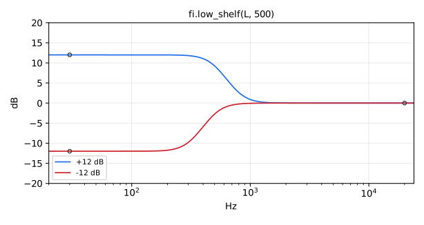
Default low shelf filter: 3rd-order Butterworth case of fi.lowshelf
(low_shelf = lowshelf(3)), boosting or cutting by L0 dB between dc and
fx. low_shelf is a standard Faust function. See fi.lowshelf for the
full documentation, including the shelf shape.
Usage
_ : low_shelf(L0,fx) : _
Where:
L0: desired level (dB) between dc andfx(boostL0>0or cutL0<0)fx: transition frequency in Hz
Test
fi = library("filters.lib");
os = library("oscillators.lib");
ba = library("basics.lib");
no = library("noises.lib");
ma = library("maths.lib");
src = os.tosc(440);
low_shelf_test = src : fi.low_shelf(6, 500);
low_shelf_slider_test = no.noise : fi.low_shelf(hslider("L0", 6, -24, 24, 0.1), hslider("fc", 500, 20, 20000, 1));
low_shelf_modulated_test = no.noise : fi.low_shelf(6, 20*pow(250, tri)) with { P = int(ma.SR/10); tri = 1 - abs(2*ba.period(P)/P - 1); };
low_shelf_jump_test = no.noise : fi.low_shelf(6, 20*pow(250, sq)) with { P = int(ma.SR/10); sq = ba.period(2*P) < P; };
(fi.)low_shelf1
First-order low shelf filter, an optimized special case of fi.lowshelf(1):
boosts or cuts by L0 dB between dc and fx.
Usage
_ : low_shelf1(L0,fx) : _
Where:
L0: desired level (dB) between dc andfx(boostL0>0or cutL0<0)fx: transition frequency in Hz
Test
fi = library("filters.lib");
os = library("oscillators.lib");
ba = library("basics.lib");
no = library("noises.lib");
ma = library("maths.lib");
src = os.tosc(440);
low_shelf1_test = fi.low_shelf1(2, 500, src);
low_shelf1_slider_test = no.noise : fi.low_shelf1(hslider("L0", 2, -24, 24, 0.1), hslider("fc", 500, 20, 20000, 1));
low_shelf1_modulated_test = no.noise : fi.low_shelf1(2, 20*pow(250, tri)) with { P = int(ma.SR/10); tri = 1 - abs(2*ba.period(P)/P - 1); };
low_shelf1_jump_test = no.noise : fi.low_shelf1(2, 20*pow(250, sq)) with { P = int(ma.SR/10); sq = ba.period(2*P) < P; };
(fi.)low_shelf1_l
First-order low shelf filter like fi.low_shelf1, but taking a LINEAR gain
G0 instead of a level in dB (avoids computing ba.db2linear at run time
when the gain is already linear).
Usage
_ : low_shelf1_l(G0,fx) : _
Where:
G0: desired linear gain between dc andfxfx: transition frequency in Hz
Test
fi = library("filters.lib");
os = library("oscillators.lib");
ba = library("basics.lib");
no = library("noises.lib");
ma = library("maths.lib");
src = os.tosc(440);
low_shelf1_l_test = fi.low_shelf1_l(2, 500, src);
low_shelf1_l_slider_test = no.noise : fi.low_shelf1_l(hslider("G0", 2, 0, 16, 0.01), hslider("fc", 500, 20, 20000, 1));
low_shelf1_l_modulated_test = no.noise : fi.low_shelf1_l(2, 20*pow(250, tri)) with { P = int(ma.SR/10); tri = 1 - abs(2*ba.period(P)/P - 1); };
low_shelf1_l_jump_test = no.noise : fi.low_shelf1_l(2, 20*pow(250, sq)) with { P = int(ma.SR/10); sq = ba.period(2*P) < P; };
(fi.)lowshelf_other_freq
Second corner frequency of a low shelf: given the shelf order N, level
L0 and transition frequency fx of fi.lowshelf(N,L0,fx), returns the
frequency at which the response returns to 0 dB (see the "Shelf Shape"
section of fi.lowshelf). This is a frequency computation, not a filter.
Usage
lowshelf_other_freq(N,L0,fx) : _
Where:
N: shelf order (odd)L0: shelf level in dBfx: transition frequency in Hz
Test
fi = library("filters.lib");
ba = library("basics.lib");
ma = library("maths.lib");
lowshelf_other_freq_test = fi.lowshelf_other_freq(3, 6, 500);
lowshelf_other_freq_slider_test = fi.lowshelf_other_freq(3, hslider("L0", 6, -24, 24, 0.1), hslider("fc", 500, 20, 20000, 1));
lowshelf_other_freq_modulated_test = fi.lowshelf_other_freq(3, 6, 20*pow(250, tri)) with { P = int(ma.SR/10); tri = 1 - abs(2*ba.period(P)/P - 1); };
lowshelf_other_freq_jump_test = fi.lowshelf_other_freq(3, 6, 20*pow(250, sq)) with { P = int(ma.SR/10); sq = ba.period(2*P) < P; };
(fi.)highshelf
Order-N "high shelf" filter (gain boost|cut above some frequency).
high_shelf is a standard Faust function.
Usage
_ : highshelf(N,Lpi,fx) : _
_ : high_shelf(L0,fx) : _ // default case (order 3)
_ : highshelf_other_freq(N,Lpi,fx) : _
Where:
N: filter order 1, 3, 5, ... (odd only, a constant numerical expression).Lpi: desired level (dB) between fx and SR/2 (boost Lpi>0 or cut Lpi<0)fx: -3dB frequency of highpass band (L0>0) or lower band (L0<0) (Use highshelf_other_freq() below to find the other one.)
The gain at dc is constrained to be 1.
See lowshelf documentation above for more details on shelf shape.
Test
fi = library("filters.lib");
os = library("oscillators.lib");
ba = library("basics.lib");
no = library("noises.lib");
ma = library("maths.lib");
src = os.tosc(440);
highshelf_test = src : fi.highshelf(3, 6, 2000);
highshelf_slider_test = no.noise : fi.highshelf(3, hslider("Lpi", 6, -24, 24, 0.1), hslider("fc", 2000, 20, 20000, 1));
highshelf_modulated_test = no.noise : fi.highshelf(3, 6, 20*pow(250, tri)) with { P = int(ma.SR/10); tri = 1 - abs(2*ba.period(P)/P - 1); };
highshelf_jump_test = no.noise : fi.highshelf(3, 6, 20*pow(250, sq)) with { P = int(ma.SR/10); sq = ba.period(2*P) < P; };
References
- See "Parametric Equalizers" above for references regarding
low_shelf,high_shelf, andpeak_eq.
(fi.)high_shelf
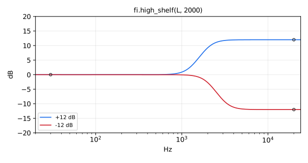
Default high shelf filter: 3rd-order Butterworth case of fi.highshelf
(high_shelf = highshelf(3)), boosting or cutting by Lpi dB between fx
and SR/2. high_shelf is a standard Faust function. See fi.highshelf
for the full documentation.
Usage
_ : high_shelf(Lpi,fx) : _
Where:
Lpi: desired level (dB) betweenfxand SR/2 (boostLpi>0or cutLpi<0)fx: transition frequency in Hz
Test
fi = library("filters.lib");
os = library("oscillators.lib");
ba = library("basics.lib");
no = library("noises.lib");
ma = library("maths.lib");
src = os.tosc(440);
high_shelf_test = src : fi.high_shelf(6, 2000);
high_shelf_slider_test = no.noise : fi.high_shelf(hslider("Lpi", 6, -24, 24, 0.1), hslider("fc", 2000, 20, 20000, 1));
high_shelf_modulated_test = no.noise : fi.high_shelf(6, 20*pow(250, tri)) with { P = int(ma.SR/10); tri = 1 - abs(2*ba.period(P)/P - 1); };
high_shelf_jump_test = no.noise : fi.high_shelf(6, 20*pow(250, sq)) with { P = int(ma.SR/10); sq = ba.period(2*P) < P; };
(fi.)high_shelf1
First-order high shelf filter, an optimized special case of
fi.highshelf(1): boosts or cuts by Lpi dB between fx and SR/2.
Usage
_ : high_shelf1(Lpi,fx) : _
Where:
Lpi: desired level (dB) betweenfxand SR/2 (boostLpi>0or cutLpi<0)fx: transition frequency in Hz
Test
fi = library("filters.lib");
os = library("oscillators.lib");
ba = library("basics.lib");
no = library("noises.lib");
ma = library("maths.lib");
src = os.tosc(440);
high_shelf1_test = fi.high_shelf1(6, 2000, src);
high_shelf1_slider_test = no.noise : fi.high_shelf1(hslider("Lpi", 6, -24, 24, 0.1), hslider("fc", 2000, 20, 20000, 1));
high_shelf1_modulated_test = no.noise : fi.high_shelf1(6, 20*pow(250, tri)) with { P = int(ma.SR/10); tri = 1 - abs(2*ba.period(P)/P - 1); };
high_shelf1_jump_test = no.noise : fi.high_shelf1(6, 20*pow(250, sq)) with { P = int(ma.SR/10); sq = ba.period(2*P) < P; };
(fi.)high_shelf1_l
First-order high shelf filter like fi.high_shelf1, but taking a LINEAR
gain Gpi instead of a level in dB.
Usage
_ : high_shelf1_l(Gpi,fx) : _
Where:
Gpi: desired linear gain betweenfxand SR/2fx: transition frequency in Hz
Test
fi = library("filters.lib");
os = library("oscillators.lib");
ba = library("basics.lib");
no = library("noises.lib");
ma = library("maths.lib");
src = os.tosc(440);
high_shelf1_l_test = fi.high_shelf1_l(2, 2000, src);
high_shelf1_l_slider_test = no.noise : fi.high_shelf1_l(hslider("Gpi", 2, 0, 16, 0.01), hslider("fc", 2000, 20, 20000, 1));
high_shelf1_l_modulated_test = no.noise : fi.high_shelf1_l(2, 20*pow(250, tri)) with { P = int(ma.SR/10); tri = 1 - abs(2*ba.period(P)/P - 1); };
high_shelf1_l_jump_test = no.noise : fi.high_shelf1_l(2, 20*pow(250, sq)) with { P = int(ma.SR/10); sq = ba.period(2*P) < P; };
(fi.)highshelf_other_freq
Second corner frequency of a high shelf: given the shelf order N, level
Lpi and transition frequency fx of fi.highshelf(N,Lpi,fx), returns
the frequency at which the response leaves 0 dB. This is a frequency
computation, not a filter.
Usage
highshelf_other_freq(N,Lpi,fx) : _
Where:
N: shelf order (odd)Lpi: shelf level in dBfx: transition frequency in Hz
Test
fi = library("filters.lib");
ba = library("basics.lib");
ma = library("maths.lib");
highshelf_other_freq_test = fi.highshelf_other_freq(3, 6, 2000);
highshelf_other_freq_slider_test = fi.highshelf_other_freq(3, hslider("Lpi", 6, -24, 24, 0.1), hslider("fc", 2000, 20, 20000, 1));
highshelf_other_freq_modulated_test = fi.highshelf_other_freq(3, 6, 20*pow(250, tri)) with { P = int(ma.SR/10); tri = 1 - abs(2*ba.period(P)/P - 1); };
highshelf_other_freq_jump_test = fi.highshelf_other_freq(3, 6, 20*pow(250, sq)) with { P = int(ma.SR/10); sq = ba.period(2*P) < P; };
(fi.)peak_eq
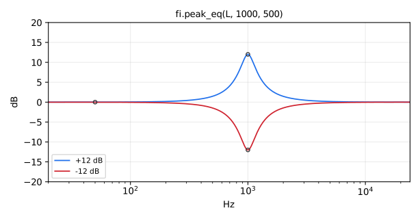
Second order "peaking equalizer" section (gain boost or cut near some frequency)
Also called a "parametric equalizer" section.
peak_eq is a standard Faust function.
Usage
_ : peak_eq(Lfx,fx,B) : _
Where:
Lfx: level (dB) at fx (boost Lfx>0 or cut Lfx<0)fx: peak frequency (Hz), clamped to [0.001, 0.499*SR]: the bandwidth prewarping divides bysin(2*PI*fx/SR), which is 0 at 0 and SR/2. Asfxgoes to 0, the peak becomes a shelf of levelLfxbelow aboutBHz.B: bandwidth of the peak in Hz (B = fx/Q): the bandwidth of the resonance (boost) or anti-resonance (cut), which is the -3 dB bandwidth about fx when |Lfx| is large
Test
fi = library("filters.lib");
os = library("oscillators.lib");
ba = library("basics.lib");
no = library("noises.lib");
ma = library("maths.lib");
src = os.tosc(440);
peak_eq_test = src : fi.peak_eq(6, 1000, 200);
peak_eq_zero_freq_test = no.noise : fi.peak_eq(6, 1000*max(0, 1 - ba.time/12000) + 1000*(ba.time >= 24000), 100);
peak_eq_slider_test = no.noise : fi.peak_eq(hslider("Lfx", 6, -24, 24, 0.1), hslider("fc", 1000, 20, 20000, 1), hslider("B", 200, 1, 5000, 1));
peak_eq_modulated_test = no.noise : fi.peak_eq(6, fx, fx/5) with { P = int(ma.SR/10); tri = 1 - abs(2*ba.period(P)/P - 1); fx = 20*pow(250, tri); };
peak_eq_jump_test = no.noise : fi.peak_eq(6, fx, fx/5) with { P = int(ma.SR/10); sq = ba.period(2*P) < P; fx = 20*pow(250, sq); };
References
- See "Parametric Equalizers" above for references regarding
low_shelf,high_shelf, andpeak_eq.
(fi.)peak_eq_cq
Constant-Q second order peaking equalizer section.
Usage
_ : peak_eq_cq(Lfx,fx,Q) : _
Where:
Lfx: level (dB) at fxfx: boost or cut frequency (Hz)Q: "Quality factor" = fx/B where B = bandwidth of peak in Hz
Test
fi = library("filters.lib");
os = library("oscillators.lib");
ba = library("basics.lib");
no = library("noises.lib");
ma = library("maths.lib");
src = os.tosc(440);
peak_eq_cq_test = src : fi.peak_eq_cq(6, 1000, 4);
peak_eq_cq_slider_test = no.noise : fi.peak_eq_cq(hslider("Lfx", 6, -24, 24, 0.1), hslider("fc", 1000, 20, 20000, 1), hslider("Q", 4, 0.5, 20, 0.01));
peak_eq_cq_modulated_test = no.noise : fi.peak_eq_cq(6, 20*pow(250, tri), 4) with { P = int(ma.SR/10); tri = 1 - abs(2*ba.period(P)/P - 1); };
peak_eq_cq_jump_test = no.noise : fi.peak_eq_cq(6, 20*pow(250, sq), 4) with { P = int(ma.SR/10); sq = ba.period(2*P) < P; };
References
- See "Parametric Equalizers" above for references regarding
low_shelf,high_shelf, andpeak_eq.
(fi.)peak_eq_rm
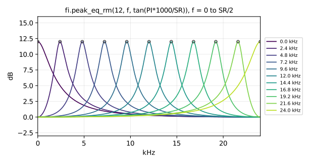
Regalia-Mitra second order peaking equalizer section:
H(z) = (1 + A(z))/2 + K (1 - A(z))/2, with A(z) the second order
allpass centered at fx and K = 10^(Lfx/20). At Lfx = 0 (K = 1) the
section is the identity. It is realized as a trapezoidal state-variable
filter, x + (K - 1)*k*bp, which stays accurate in single precision at low
fx and near the Nyquist limit, and continuous when fx jumps or moves at
audio rate: its states hold k*bp, at the output level.
Usage
_ : peak_eq_rm(Lfx,fx,tanPiBT) : _
Where:
Lfx: level (dB) at fxfx: boost or cut frequency (Hz), from 0 (where the section becomes a first-order shelf) toma.SR/2(the mirror image of that shelf, at the Nyquist limit). Abovema.SR/4the section runs mirrored, as intf2_tpt, so that a peak near the Nyquist limit is as accurate as one near 0 HztanPiBT:tan(PI*B/SR), where B = -3dB bandwidth (Hz) when 10^(Lfx/20) = 0 ~ PI*B/SR for narrow bandwidths B
Test
fi = library("filters.lib");
os = library("oscillators.lib");
ma = library("maths.lib");
ba = library("basics.lib");
no = library("noises.lib");
src = os.tosc(440);
peak_eq_rm_test = src : fi.peak_eq_rm(6, 1000, tan(ma.PI*200/ma.SR));
peak_eq_rm_slider_test = no.noise : fi.peak_eq_rm(hslider("Lfx", 6, -24, 24, 0.1), hslider("fc", 1000, 20, 20000, 1), tan(ma.PI*hslider("B", 200, 1, 5000, 1)/ma.SR));
peak_eq_rm_modulated_test = no.noise : fi.peak_eq_rm(6, fx, tan(ma.PI*fx/5/ma.SR)) with { P = int(ma.SR/10); tri = 1 - abs(2*ba.period(P)/P - 1); fx = 20*pow(250, tri); };
peak_eq_rm_jump_test = no.noise : fi.peak_eq_rm(6, fx, tan(ma.PI*fx/5/ma.SR)) with { P = int(ma.SR/10); sq = ba.period(2*P) < P; fx = 20*pow(250.0, sq); };
peak_eq_rm_unity_test = no.noise : fi.peak_eq_rm(0, 1000, tan(ma.PI*200/ma.SR));
peak_eq_rm_audio_modulated_test = 0.1*no.noise : fi.peak_eq_rm(6, fc, tan(ma.PI*fc/10/ma.SR)) with { fc = max(20, 1000*(1 + 0.9*os.tosc(500))); };
peak_eq_rm_dc_test = no.noise : fi.peak_eq_rm(6, 0, tan(ma.PI*200/ma.SR));
peak_eq_rm_nyquist_test = no.noise : fi.peak_eq_rm(6, ma.SR/2, tan(ma.PI*200/ma.SR));
peak_eq_rm_high_test = no.noise : fi.peak_eq_rm(6, ma.SR/2 - 100, tan(ma.PI*200/ma.SR));
peak_eq_rm_mirror_modulated_test = no.noise : fi.peak_eq_rm(6, fx, tan(ma.PI*1000/ma.SR)) with { P = int(ma.SR/10); tri = 1 - abs(2*ba.period(P)/P - 1); fx = ma.SR*(0.1 + 0.35*tri); };
peak_eq_rm_mirror_jump_test = no.noise : fi.peak_eq_rm(6, fx, tan(ma.PI*1000/ma.SR)) with { P = int(ma.SR/10); sq = ba.period(2*P) < P; fx = ma.SR*select2(sq, 0.1, 0.45); };
peak_eq_rm_low_jump_test = no.noise : fi.peak_eq_rm(12, fx, tan(ma.PI*1000/ma.SR)) with { P = int(ma.SR/10); sq = ba.period(2*P) < P; fx = select2(sq, 2400, 24); };
References
P.A. Regalia, S.K. Mitra, and P.P. Vaidyanathan, "The Digital All-Pass Filter: A Versatile Signal Processing Building Block" Proceedings of the IEEE, 76(1):19-37, Jan. 1988. (See pp. 29-30.) See also "Parametric Equalizers" above for references on shelf and peaking equalizers in general.
Julius O. Smith III, "Digital State-Variable Filters", for the trapezoidal (TPT) state-variable filter this section runs on, and its bell output: https://ccrma.stanford.edu/~jos/svf/Output_Mixing_Nine_Filter.html
(fi.)spectral_tilt
Spectral tilt filter, providing an arbitrary spectral rolloff factor alpha in (-1,1), where -1 corresponds to one pole (-6 dB per octave), and +1 corresponds to one zero (+6 dB per octave). In other words, alpha is the slope of the ln magnitude versus ln frequency. For a "pinking filter" (e.g., to generate 1/f noise from white noise), set alpha to -1/2.
Usage
_ : spectral_tilt(N,f0,bw,alpha) : _
Where:
N: desired integer filter order, at least 2 (fixed at compile time)f0: lower frequency limit for desired roll-off band > 0bw: bandwidth of desired roll-off bandalpha: slope of roll-off desired in nepers per neper, between -1 and 1 (ln mag / ln radian freq)
Test
fi = library("filters.lib");
os = library("oscillators.lib");
ba = library("basics.lib");
no = library("noises.lib");
ma = library("maths.lib");
src = os.tosc(440);
spectral_tilt_test = src : fi.spectral_tilt(4, 200, 2000, -0.5);
spectral_tilt_slider_test = no.noise : fi.spectral_tilt(4, hslider("f0", 200, 20, 2000, 1), hslider("bw", 2000, 100, 10000, 1), hslider("alpha", -0.5, -1, 1, 0.01));
spectral_tilt_modulated_test = no.noise : fi.spectral_tilt(4, 200, 2000, -1 + 2*tri) with { P = int(ma.SR/10); tri = 1 - abs(2*ba.period(P)/P - 1); };
spectral_tilt_jump_test = no.noise : fi.spectral_tilt(4, 200, 2000, -1 + 2*sq) with { P = int(ma.SR/10); sq = ba.period(2*P) < P; };
Example test program
See dm.spectral_tilt_demo and the documentation for no.pink_noise.
References
J.O. Smith and H.F. Smith, "Closed Form Fractional Integration and Differentiation via Real Exponentially Spaced Pole-Zero Pairs", arXiv.org publication arXiv:1606.06154 [cs.CE], June 7, 2016, http://arxiv.org/abs/1606.06154
(fi.)levelfilter
Dynamic level lowpass filter.
levelfilter is a standard Faust function.
Usage
_ : levelfilter(L,freq) : _
Where:
L: level, linear between 0 and 1 (not in dB: a negative value gives NaN): 1 passes the input unchanged, smaller values lowpass it more. The gain is L^(4/3) at the Nyquist limit (SR/2), and 1 - L + L^(4/3) (within 1 dB of unity) at dcfreq: corner frequency (-3dB point when L = 0) usually set to fundamental freq
See levelfilterN for N such filters in series.
Test
fi = library("filters.lib");
os = library("oscillators.lib");
ba = library("basics.lib");
no = library("noises.lib");
ma = library("maths.lib");
src = os.tosc(440);
levelfilter_test = fi.levelfilter(0.1, 200, src);
levelfilter_slider_test = fi.levelfilter(hslider("L", 0.1, 0, 1, 0.01), hslider("fc", 200, 20, 20000, 1), no.noise);
levelfilter_modulated_test = fi.levelfilter(0.1, 20*pow(250, tri), no.noise) with { P = int(ma.SR/10); tri = 1 - abs(2*ba.period(P)/P - 1); };
levelfilter_jump_test = fi.levelfilter(0.1, 20*pow(250, sq), no.noise) with { P = int(ma.SR/10); sq = ba.period(2*P) < P; };
levelfilter_dc_test = fi.levelfilter(0.1, 200, 1);
References
(fi.)levelfilterN
Dynamic level lowpass filter.
Usage
_ : levelfilterN(N,freq,L) : _
Where:
N: number oflevelfilterin series, each with the levelL^(1/N), a constant numerical expressionfreq: corner frequency of eachlevelfilter, usually set to fundamental freqL: level, linear between 0 and 1 (seelevelfilter); the cascade has the same gain at the Nyquist limit as onelevelfilter
Test
fi = library("filters.lib");
os = library("oscillators.lib");
ba = library("basics.lib");
no = library("noises.lib");
ma = library("maths.lib");
src = os.tosc(440);
levelfilterN_test = src : fi.levelfilterN(3, 200, 0.1);
levelfilterN_slider_test = no.noise : fi.levelfilterN(3, hslider("fc", 200, 20, 20000, 1), hslider("L", 0.1, 0, 1, 0.01));
levelfilterN_modulated_test = no.noise : fi.levelfilterN(3, 20*pow(250, tri), 0.1) with { P = int(ma.SR/10); tri = 1 - abs(2*ba.period(P)/P - 1); };
levelfilterN_jump_test = no.noise : fi.levelfilterN(3, 20*pow(250, sq), 0.1) with { P = int(ma.SR/10); sq = ba.period(2*P) < P; };
levelfilterN_nyquist_test = 1 - 2*ba.period(2) : fi.levelfilterN(3, 200, 0.1);
References
Mth-Octave Filter-Banks
Mth-octave filter-banks split the input signal into a bank of parallel signals, one
for each spectral band. They are related to the Mth-Octave Spectrum-Analyzers in
analysis.lib.
The documentation of this library contains more details about the implementation.
The parameters are:
M: number of band-slices per octave (>=1), a constant numerical expressionN: total number of bands (>2), a constant numerical expressionftop: upper bandlimit of the Mth-octave bands (<SR/2)
In addition to the Mth-octave output signals, there is a highpass signal containing frequencies from ftop to SR/2, and a "dc band" lowpass signal containing frequencies from 0 (dc) up to the start of the Mth-octave bands. Thus, the N output signals are
highpass(ftop), MthOctaveBands(M,N-2,ftop), dcBand(ftop*2^(-(N-2)/M))
A Filter-Bank is defined here as a signal bandsplitter having the property that summing its output signals gives an allpass-filtered version of the filter-bank input signal. A more conventional term for this is an "allpass-complementary filter bank". If the allpass filter is a pure delay (and possible scaling), the filter bank is said to be a "perfect-reconstruction filter bank" (see Vaidyanathan-1993 cited below for details). A "graphic equalizer", in which band signals are scaled by gains and summed, should be based on a filter bank.
The filter-banks below are implemented as Butterworth or Elliptic spectrum-analyzers followed by delay equalizers that make them allpass-complementary.
Increasing Channel Isolation
Go to higher filter orders - see Regalia et al. or Vaidyanathan (cited below) regarding the construction of more aggressive recursive filter-banks using elliptic or Chebyshev prototype filters.
References
- "Tree-structured complementary filter banks using all-pass sections", Regalia et al., IEEE Trans. Circuits & Systems, CAS-34:1470-1484, Dec. 1987
- "Multirate Systems and Filter Banks", P. Vaidyanathan, Prentice-Hall, 1993
- Elementary filter theory: https://ccrma.stanford.edu/~jos/filters/
(fi.)mth_octave_filterbank[n], (fi.)mth_octave_filterbank
Allpass-complementary filter banks based on Butterworth band-splitting.
For Butterworth band-splits, the needed delay equalizer is easily found.
Sections whose crossover is at or above tpt_df_fmin (2304 Hz in single
precision, 0 in double) are direct form, the others trapezoidal: see
mth_octave_filterbank_tpt_df.
Usage
_ : mth_octave_filterbank(O,M,ftop,N) : par(i,N,_)     // Oth-order
_ : mth_octave_filterbank_alt(O,M,ftop,N) : par(i,N,_) // dc-inverted version
Also for convenience:
_ : mth_octave_filterbank3(M,ftop,N) : par(i,N,_) // 3rd-order Butterworth
_ : mth_octave_filterbank5(M,ftop,N) : par(i,N,_) // 5th-order Butterworth
mth_octave_filterbank_default = mth_octave_filterbank5;
Where:
O: order of filter used to split each frequency band into two, a constant numerical expressionM: number of band-slices per octave, a constant numerical expressionftop: highest band-split crossover frequency (e.g., 20 kHz)N: total number of bands (including dc and Nyquist), a constant numerical expression
Test
fi = library("filters.lib");
os = library("oscillators.lib");
sig = os.tosc(440);
mth_octave_filterbank_test = sig : fi.mth_octave_filterbank(3, 2, 8000, 2);
(fi.)mth_octave_filterbank_tpt_df, (fi.)mth_octave_filterbank_alt_tpt_df
mth_octave_filterbank and mth_octave_filterbank_alt with an explicit
cutoff limit L, as filterbank_tpt_df is to filterbank:
mth_octave_filterbank(O,M,ftop,N) is
mth_octave_filterbank_tpt_df(tpt_df_fmin,O,M,ftop,N), and likewise for
the _alt version (and so for mth_octave_filterbank3, 5 and
_default).
Usage
_ : mth_octave_filterbank_tpt_df(L,O,M,ftop,N) : par(i,N,_)
_ : mth_octave_filterbank_alt_tpt_df(L,O,M,ftop,N) : par(i,N,_)
Where:
L: cutoff limit in Hz, usuallytpt_df_fmin;L <= 0selects the direct form andL >= ma.MAXthe trapezoidal form for every crossoverO,M,ftop,N: as formth_octave_filterbank
Test
fi = library("filters.lib");
no = library("noises.lib");
mth_octave_filterbank_tpt_df_test = no.noise : fi.mth_octave_filterbank_tpt_df(fi.tpt_df_fmin, 5, 1, 10000, 10);
mth_octave_filterbank_tpt_df_sum_test = no.noise : fi.mth_octave_filterbank_tpt_df(fi.tpt_df_fmin, 5, 1, 10000, 10) :> _;
mth_octave_filterbank_alt_tpt_df_test = no.noise : fi.mth_octave_filterbank_alt_tpt_df(fi.tpt_df_fmin, 3, 2, 8000, 10);
mth_octave_filterbank_alt_tpt_df_sum_test = no.noise : fi.mth_octave_filterbank_alt_tpt_df(fi.tpt_df_fmin, 5, 2, 8000, 10) :> _;
(fi.)mth_octave_filterbank_alt
Usage
_ : mth_octave_filterbank_alt(O,M,ftop,N) : par(i,N,_)
Where:
O: filter order used to split each bandM: number of band-slices per octaveftop: highest band-split crossover frequencyN: total number of bands
Test
fi = library("filters.lib");
os = library("oscillators.lib");
no = library("noises.lib");
sig = os.tosc(440);
mth_octave_filterbank_alt_test = sig : fi.mth_octave_filterbank_alt(3, 2, 8000, 2);
mth_octave_filterbank_alt_bands_test = sig : fi.mth_octave_filterbank_alt(3, 2, 8000, 5);
mth_octave_filterbank_alt_o5_sum_test = no.noise : fi.mth_octave_filterbank_alt(5, 2, 8000, 5) :> _;
(fi.)mth_octave_filterbank3
Usage
_ : mth_octave_filterbank3(M,ftop,N) : par(i,N,_)
Where:
M: number of band-slices per octaveftop: highest band-split crossover frequencyN: total number of bands
Test
fi = library("filters.lib");
os = library("oscillators.lib");
sig = os.tosc(440);
mth_octave_filterbank3_test = sig : fi.mth_octave_filterbank3(2, 8000, 2);
mth_octave_filterbank3_bands_test = sig : fi.mth_octave_filterbank3(2, 8000, 5);
(fi.)mth_octave_filterbank5
Usage
_ : mth_octave_filterbank5(M,ftop,N) : par(i,N,_)
Where:
M: number of band-slices per octaveftop: highest band-split crossover frequencyN: total number of bands
Test
fi = library("filters.lib");
os = library("oscillators.lib");
sig = os.tosc(440);
mth_octave_filterbank5_test = sig : fi.mth_octave_filterbank5(2, 8000, 2);
(fi.)mth_octave_filterbank_default
Default Mth-octave filter bank: the 5th-order Butterworth case of
fi.mth_octave_filterbank (mth_octave_filterbank_default =
mth_octave_filterbank5). See fi.mth_octave_filterbank[n] for the full
documentation.
Usage
_ : mth_octave_filterbank_default(M,ftop,N) : par(i,N,_)
Where:
M: number of band-slices per octave (a constant numerical expression)ftop: highest band-split crossover frequency in HzN: total number of bands, including dc and Nyquist (a constant numerical expression)
Test
fi = library("filters.lib");
os = library("oscillators.lib");
sig = os.tosc(440);
mth_octave_filterbank_default_test = sig : fi.mth_octave_filterbank_default(2, 8000, 2);
Arbitrary-Crossover Filter-Banks and Spectrum Analyzers
These are similar to the Mth-octave analyzers above, except that the band-split frequencies are passed explicitly as arguments.
(fi.)filterbank
Filter bank.
filterbank is a standard Faust function.
Sections whose crossover is at or above tpt_df_fmin (2304 Hz in single
precision, 0 in double) are direct form, the others trapezoidal: see
filterbank_tpt_df.
Usage
_ : filterbank(O,freqs) : par(i,ba.count(freqs)+1,_) // Butterworth band-splits
Where:
O: band-split filter order (odd integer required for filterbank[i], a constant numerical expression)freqs: (fc1,fc2,...,fcNs) [in numerically ascending order], where Ns=N-1 is the number of octave band-splits (total number of bands N=Ns+1, the number of outputs).
If frequencies are listed explicitly as arguments, enclose them in parens:
_ : filterbank(3,(fc1,fc2)) : _,_,_
Test
fi = library("filters.lib");
os = library("oscillators.lib");
src = os.tosc(440);
filterbank_test = src : fi.filterbank(3, (500, 2000));
(fi.)filterbank_tpt_df
filterbank with an explicit cutoff limit L: the band splits and delay
equalizers whose crossover is below L use trapezoidal sections, the
others the cheaper direct-form sections (lowpass_tpt_df,
highpass_plus_lowpass_tpt_df). filterbank(O,freqs) is
filterbank_tpt_df(tpt_df_fmin,O,freqs): trapezoidal below 2304 Hz in
single precision, direct form everywhere in double precision. Each
section is compiled in one form only when its crossover is a constant;
for crossovers that vary (sliders), pass L = ma.MAX (trapezoidal) or
L = 0 (direct form), or both forms run.
Usage
_ : filterbank_tpt_df(L,O,freqs) : par(i,ba.count(freqs)+1,_)
Where:
L: cutoff limit in Hz, usuallytpt_df_fmin;L <= 0selects the direct form andL >= ma.MAXthe trapezoidal form for every crossoverO,freqs: as forfilterbank
Test
fi = library("filters.lib");
no = library("noises.lib");
ba = library("basics.lib");
ma = library("maths.lib");
filterbank_tpt_df_test = no.noise : fi.filterbank_tpt_df(fi.tpt_df_fmin, 3, (50, 500, 4000));
filterbank_tpt_df_o5_sum_test = no.noise : fi.filterbank_tpt_df(fi.tpt_df_fmin, 5, (50, 500, 4000)) :> _;
filterbank_tpt_df_slider_test = no.noise : fi.filterbank_tpt_df(fi.tpt_df_fmin, 3, (hslider("f1", 500, 20, 10000, 1), hslider("f2", 4000, 20, 20000, 1)));
filterbank_tpt_df_modulated_test = no.noise : fi.filterbank_tpt_df(0, 3, (f1, 4*f1)) with { P = int(ma.SR/10); tri = 1 - abs(2*ba.period(P)/P - 1); f1 = 2500*pow(2, tri); };
filterbank_tpt_df_jump_test = no.noise : fi.filterbank_tpt_df(ma.MAX, 3, (f1, 4*f1)) with { P = int(ma.SR/10); sq = ba.period(2*P) < P; f1 = 100*pow(10, sq); };
(fi.)filterbanki
Inverted-dc filter bank.
Sections whose crossover is at or above tpt_df_fmin (2304 Hz in single
precision, 0 in double) are direct form, the others trapezoidal: see
filterbanki_tpt_df.
Usage
_ : filterbanki(O,freqs) : par(i,ba.count(freqs)+1,_) // Inverted-dc version
Where:
O: band-split filter order (odd integer required forfilterbank[i], a constant numerical expression)freqs: (fc1,fc2,...,fcNs) [in numerically ascending order], where Ns=N-1 is the number of octave band-splits (total number of bands N=Ns+1, the number of outputs).
If frequencies are listed explicitly as arguments, enclose them in parens:
_ : filterbanki(3,(fc1,fc2)) : _,_,_
Test
fi = library("filters.lib");
os = library("oscillators.lib");
no = library("noises.lib");
src = os.tosc(440);
filterbanki_test = src : fi.filterbanki(3, (500, 2000));
filterbanki_o5_sum_test = no.noise : fi.filterbanki(5, (500, 1000, 2000)) :> _;
(fi.)filterbanki_tpt_df
filterbanki with an explicit cutoff limit L, as filterbank_tpt_df
is to filterbank: filterbanki(O,freqs) is
filterbanki_tpt_df(tpt_df_fmin,O,freqs).
Usage
_ : filterbanki_tpt_df(L,O,freqs) : par(i,ba.count(freqs)+1,_)
Where:
L: cutoff limit in Hz, usuallytpt_df_fmin;L <= 0selects the direct form andL >= ma.MAXthe trapezoidal form for every crossoverO,freqs: as forfilterbanki
Test
fi = library("filters.lib");
no = library("noises.lib");
ba = library("basics.lib");
ma = library("maths.lib");
filterbanki_tpt_df_test = no.noise : fi.filterbanki_tpt_df(fi.tpt_df_fmin, 3, (50, 500, 4000));
filterbanki_tpt_df_o5_sum_test = no.noise : fi.filterbanki_tpt_df(fi.tpt_df_fmin, 5, (50, 500, 4000)) :> _;
filterbanki_tpt_df_slider_test = no.noise : fi.filterbanki_tpt_df(fi.tpt_df_fmin, 3, (hslider("f1", 500, 20, 10000, 1), hslider("f2", 4000, 20, 20000, 1)));
filterbanki_tpt_df_modulated_test = no.noise : fi.filterbanki_tpt_df(0, 3, (f1, 4*f1)) with { P = int(ma.SR/10); tri = 1 - abs(2*ba.period(P)/P - 1); f1 = 2500*pow(2, tri); };
filterbanki_tpt_df_jump_test = no.noise : fi.filterbanki_tpt_df(ma.MAX, 3, (f1, 4*f1)) with { P = int(ma.SR/10); sq = ba.period(2*P) < P; f1 = 100*pow(10, sq); };
State Variable Filters
References
- Solving the continuous SVF equations using trapezoidal integration
- https://cytomic.com/files/dsp/SvfLinearTrapOptimised2.pdf
(fi.)svf
An environment with lp, bp, hp, notch, peak, ap, bell, ls, hs SVF based filters.
All filters have freq and Q parameters, the bell, ls, hs ones also have a gain third parameter.
Usage
_ : svf.lp(freq, Q) : _
_ : svf.bp(freq, Q) : _
_ : svf.hp(freq, Q) : _
_ : svf.notch(freq, Q) : _
_ : svf.peak(freq, Q) : _
_ : svf.ap(freq, Q) : _
_ : svf.bell(freq, Q, gain) : _
_ : svf.ls(freq, Q, gain) : _
_ : svf.hs(freq, Q, gain) : _
Where:
freq: cut frequency in Hz, clamped to [0, 0.499*SR]: 0 holds the filter's states (see the section Digital Filter Sections Specified as Analog Filter Sections)Q: quality factorgain: gain in dB (bell,lsandhsonly)
Method
Andrew Simper's trapezoidal state-variable filter: the bilinear transform
of the analog state-variable filter, prewarped at freq, whose outputs
are mixed into the nine responses. The delay-free loop is solved for the
highpass first, so that each state is updated by adding a small
increment. Solving it for the bandpass first, as in Simper's listings,
multiplies a state by 1/(1 + g*(g+k)), close to 1 at a low cutoff, and
loses more than two digits of the damping in single precision: a 20 Hz
lowpass with Q = 10 at 192 kHz was 8.8e-4 off its double-precision
output, and is now 3.7e-6 off. See the section
Digital Filter Sections Specified as Analog Filter Sections
and https://ccrma.stanford.edu/~jos/svf/Numerical_Precision_Low_Corner.html.
Test
fi = library("filters.lib");
os = library("oscillators.lib");
ba = library("basics.lib");
no = library("noises.lib");
ma = library("maths.lib");
sig = os.tosc(440);
svf_lp_test = fi.svf.lp(1000, 0.707, sig);
svf_lp_lowfc_test = no.noise : fi.svf.lp(5, 10);
svf_bp_lowfc_test = no.noise : fi.svf.bp(20, 30);
svf_nyquist_test = no.noise : fi.svf.lp(0.6*ma.SR, 1);
svf_slider_test = no.noise : fi.svf.bell(hslider("fc", 1000, 20, 20000, 1), hslider("Q", 0.707, 0.5, 20, 0.01), hslider("gain", 6, -24, 24, 0.1));
svf_modulated_test = no.noise : fi.svf.lp(20*pow(250, tri), 0.707) with { P = int(ma.SR/10); tri = 1 - abs(2*ba.period(P)/P - 1); };
svf_jump_test = no.noise : fi.svf.lp(20*pow(250, sq), 0.707) with { P = int(ma.SR/10); sq = ba.period(2*P) < P; };
svf_bp_test = fi.svf.bp(1000, 0.707, sig);
svf_hp_test = fi.svf.hp(1000, 0.707, sig);
svf_notch_test = fi.svf.notch(1000, 0.707, sig);
svf_peak_test = fi.svf.peak(1000, 0.707, sig);
svf_ap_test = fi.svf.ap(1000, 0.707, sig);
svf_bell_test = fi.svf.bell(1000, 0.707, 6, sig);
svf_ls_test = fi.svf.ls(500, 0.707, 6, sig);
svf_hs_test = fi.svf.hs(3000, 0.707, 6, sig);
svf_audio_modulated_test = 0.1*no.noise <: fi.svf.lp(fc, 10), fi.svf.bp(fc, 10), fi.svf.hp(fc, 10) with { fc = max(20, 1000*(1 + 0.9*os.tosc(500))); };
(fi.)svf_morph
An SVF-based filter that can smoothly morph between being lowpass, bandpass, and highpass.
Usage
_ : svf_morph(freq, Q, blend) : _
Where:
freq: cutoff frequencyQ: quality factorblend: [0..2] continuous, where 0 islowpass, 1 isbandpass, and 2 ishighpass. For performance, the value is not clamped to [0..2].
Test
fi = library("filters.lib");
os = library("oscillators.lib");
ba = library("basics.lib");
no = library("noises.lib");
ma = library("maths.lib");
sig = os.tosc(440);
svf_morph_test = fi.svf_morph(1000, 0.707, 1, sig);
svf_morph_slider_test = fi.svf_morph(hslider("fc", 1000, 20, 20000, 1), hslider("Q", 0.707, 0.5, 20, 0.01), hslider("blend", 1, 0, 2, 0.01), no.noise);
svf_morph_modulated_test = fi.svf_morph(20*pow(250, tri), 0.707, 2*tri, no.noise) with { P = int(ma.SR/10); tri = 1 - abs(2*ba.period(P)/P - 1); };
svf_morph_jump_test = fi.svf_morph(20*pow(250, sq), 0.707, 2*sq, no.noise) with { P = int(ma.SR/10); sq = ba.period(2*P) < P; };
Example test program
process = no.noise : svf_morph(freq, q, blend)
with {
  blend = hslider("Blend", 0, 0, 2, .01) : si.smoo;
  q = hslider("Q", 1, 0.1, 10, .01) : si.smoo;
  freq = hslider("freq", 5000, 100, 18000, 1) : si.smoo;
};
References
(fi.)svf_notch_morph
An SVF-based notch-filter that can smoothly morph between being lowpass, notch, and highpass.
Usage
_ : svf_notch_morph(freq, Q, blend) : _
Where:
freq: cutoff frequencyQ: quality factorblend: [0..2] continuous, where 0 islowpass, 1 isnotch, and 2 ishighpass. For performance, the value is not clamped to [0..2].
Test
fi = library("filters.lib");
os = library("oscillators.lib");
ba = library("basics.lib");
no = library("noises.lib");
ma = library("maths.lib");
sig = os.tosc(440);
svf_notch_morph_test = fi.svf_notch_morph(1000, 0.707, 1, sig);
svf_notch_morph_slider_test = fi.svf_notch_morph(hslider("fc", 1000, 20, 20000, 1), hslider("Q", 0.707, 0.5, 20, 0.01), hslider("blend", 1, 0, 2, 0.01), no.noise);
svf_notch_morph_modulated_test = fi.svf_notch_morph(20*pow(250, tri), 0.707, 2*tri, no.noise) with { P = int(ma.SR/10); tri = 1 - abs(2*ba.period(P)/P - 1); };
svf_notch_morph_jump_test = fi.svf_notch_morph(20*pow(250, sq), 0.707, 2*sq, no.noise) with { P = int(ma.SR/10); sq = ba.period(2*P) < P; };
Example test program
process = no.noise : svf_notch_morph(freq, q, blend)
with {
  blend = hslider("Blend", 0, 0, 2, .01) : si.smoo;
  q = hslider("Q", 1, 0.1, 10, .01) : si.smoo;
  freq = hslider("freq", 5000, 100, 18000, 1) : si.smoo;
};
References
(fi.)SVFTPT
Topology-preserving transform implementation following Zavalishin's method.
Outputs: lowpass, highpass, bandpass, normalised bandpass, notch, allpass, peaking.
Each individual output can be recalled with its name in the environment as in:
SVFTPT.LP2(1000.0, .707).
The 7 outputs can be recalled by using SVF name as in:
SVFTPT.SVF(1000.0, .707).
Even though the implementation is different, the characteristics of this
filter are comparable to those of the svf environment in this library.
Usage:
_ : SVFTPT.SVF(CF, Q) : si.bus(7)
_ : SVFTPT.LP2(CF, Q) : _
_ : SVFTPT.HP2(CF, Q) : _
_ : SVFTPT.BP2(CF, Q) : _
_ : SVFTPT.BP2Norm(CF, Q) : _
_ : SVFTPT.Notch2(CF, Q) : _
_ : SVFTPT.AP2(CF, Q) : _
_ : SVFTPT.Peaking2(CF, Q) : _
Where:
CF: cutoff in HzQ: resonance
Test
fi = library("filters.lib");
os = library("oscillators.lib");
ba = library("basics.lib");
no = library("noises.lib");
ma = library("maths.lib");
sig = os.tosc(440);
SVFTPT_SVF_test = fi.SVFTPT.SVF(1000, 0.707, sig);
SVFTPT_slider_test = fi.SVFTPT.SVF(hslider("fc", 1000, 20, 20000, 1), hslider("Q", 0.707, 0.5, 20, 0.01), no.noise);
SVFTPT_modulated_test = fi.SVFTPT.SVF(20*pow(250, tri), 0.707, no.noise) with { P = int(ma.SR/10); tri = 1 - abs(2*ba.period(P)/P - 1); };
SVFTPT_jump_test = fi.SVFTPT.SVF(20*pow(250, sq), 0.707, no.noise) with { P = int(ma.SR/10); sq = ba.period(2*P) < P; };
SVFTPT_LP2_test = fi.SVFTPT.LP2(1000, 0.707, sig);
SVFTPT_HP2_test = fi.SVFTPT.HP2(1000, 0.707, sig);
SVFTPT_BP2_test = fi.SVFTPT.BP2(1000, 0.707, sig);
SVFTPT_BP2Norm_test = fi.SVFTPT.BP2Norm(1000, 0.707, sig);
SVFTPT_Notch2_test = fi.SVFTPT.Notch2(1000, 0.707, sig);
SVFTPT_AP2_test = fi.SVFTPT.AP2(1000, 0.707, sig);
SVFTPT_Peaking2_test = fi.SVFTPT.Peaking2(1000, 0.707, sig);
(fi.)dynamicSmoothing
Adaptive smoother based on Andy Simper's paper.
This filter uses both the lowpass and bandpass outputs of a state-variable filter. The lowpass is used to smooth out the input signal, the bandpass, which is a smoothed out version of the highpass, provides information on the rate of change of the input. Hence, the bandpass signal can be used to adjust the cutoff of the filter to quickly follow the input's fast and large variations while effectively filtering out local perturbations.
This implementation does not use an approximation for the CF computation, and it deploys guards to prevent overshooting with extreme sensitivity values.
Usage:
_ : dynamicSmoothing(sensitivity, baseCF) : _
Where:
sensitivity: sensitivity to changes in the input signal. The range is, theoretically, from 0 to INF, though anything between 0.0 and 1.0 should be reasonablebaseCF: cutoff frequency, in Hz, when there is no variation in the input signal
Test
fi = library("filters.lib");
os = library("oscillators.lib");
ba = library("basics.lib");
no = library("noises.lib");
ma = library("maths.lib");
sig = os.tosc(440);
dynamicSmoothing_test = fi.dynamicSmoothing(0.5, 500, sig);
dynamicSmoothing_slider_test = fi.dynamicSmoothing(hslider("sensitivity", 0.5, 0, 1, 0.01), hslider("fc", 500, 20, 20000, 1), no.noise);
dynamicSmoothing_modulated_test = fi.dynamicSmoothing(0.5, 20*pow(250, tri), no.noise) with { P = int(ma.SR/10); tri = 1 - abs(2*ba.period(P)/P - 1); };
dynamicSmoothing_jump_test = fi.dynamicSmoothing(0.5, 20*pow(250, sq), no.noise) with { P = int(ma.SR/10); sq = ba.period(2*P) < P; };
References
(fi.)oneEuro
The One Euro Filter (1€ Filter) is an adaptive lowpass filter. This kind of filter is commonly used in object-tracking, not necessarily audio processing.
Usage
_ : oneEuro(derivativeCutoff, beta, minCutoff) : _
Where:
derivativeCutoff: Used to filter the first derivative of the input. 1 Hz is a good default.beta: "Speed" parameter where higher values reduce latency.minCutoff: Minimum cutoff frequency in Hz. Lower values remove more jitter.
Test
fi = library("filters.lib");
os = library("oscillators.lib");
ba = library("basics.lib");
no = library("noises.lib");
ma = library("maths.lib");
sig = os.tosc(440);
oneEuro_test = sig : fi.oneEuro(1, 0.5, 5);
oneEuro_slider_test = no.noise : fi.oneEuro(hslider("derivativeCutoff", 1, 0.1, 10, 0.1), hslider("beta", 0.5, 0, 1, 0.01), hslider("minCutoff", 5, 0.1, 50, 0.1));
oneEuro_modulated_test = no.noise : fi.oneEuro(1, 0.5, pow(50, tri)) with { P = int(ma.SR/10); tri = 1 - abs(2*ba.period(P)/P - 1); };
oneEuro_jump_test = no.noise : fi.oneEuro(1, 0.5, pow(50, sq)) with { P = int(ma.SR/10); sq = ba.period(2*P) < P; };
References
Linkwitz-Riley 4th-order 2-way, 3-way, and 4-way crossovers
The Linkwitz-Riley (LR) crossovers are designed to produce a fully-flat magnitude response when their outputs are combined. The 4th-order LR filters (LR4) have a 24dB/octave slope and they are rather popular audio crossovers used in multi-band processing.
The LR4 can be constructed by cascading two second-order Butterworth filters. For the second-order Butterworth filters, we will use the SVF filter implemented above by setting the Q-factor to 1.0 / sqrt(2.0). These will be cascaded in pairs to build the LR4 highpass and lowpass. For the phase correction, we will use the 2nd-order Butterworth allpass.
References
Zavalishin, Vadim. "The art of VA filter design." Native Instruments, Berlin, Germany (2012).
(fi.)lowpassLR4
4th-order Linkwitz-Riley lowpass.
Usage
_ : lowpassLR4(cf) : _
Where:
cf: lowpass cutoff in Hz
Test
fi = library("filters.lib");
os = library("oscillators.lib");
ba = library("basics.lib");
no = library("noises.lib");
ma = library("maths.lib");
src = os.tosc(440);
lowpassLR4_test = src : fi.lowpassLR4(1000);
lowpassLR4_slider_test = no.noise : fi.lowpassLR4(hslider("fc", 1000, 20, 20000, 1));
lowpassLR4_modulated_test = no.noise : fi.lowpassLR4(20*pow(250, tri)) with { P = int(ma.SR/10); tri = 1 - abs(2*ba.period(P)/P - 1); };
lowpassLR4_jump_test = no.noise : fi.lowpassLR4(20*pow(250, sq)) with { P = int(ma.SR/10); sq = ba.period(2*P) < P; };
(fi.)highpassLR4
4th-order Linkwitz-Riley highpass.
Usage
_ : highpassLR4(cf) : _
Where:
cf: highpass cutoff in Hz
Test
fi = library("filters.lib");
os = library("oscillators.lib");
ba = library("basics.lib");
no = library("noises.lib");
ma = library("maths.lib");
src = os.tosc(440);
highpassLR4_test = src : fi.highpassLR4(1000);
highpassLR4_slider_test = no.noise : fi.highpassLR4(hslider("fc", 1000, 20, 20000, 1));
highpassLR4_modulated_test = no.noise : fi.highpassLR4(20*pow(250, tri)) with { P = int(ma.SR/10); tri = 1 - abs(2*ba.period(P)/P - 1); };
highpassLR4_jump_test = no.noise : fi.highpassLR4(20*pow(250, sq)) with { P = int(ma.SR/10); sq = ba.period(2*P) < P; };
(fi.)crossover2LR4
Two-way 4th-order Linkwitz-Riley crossover.
Usage
_ : crossover2LR4(cf) : si.bus(2)
Where:
cf: crossover split cutoff in Hz
Test
fi = library("filters.lib");
os = library("oscillators.lib");
ba = library("basics.lib");
no = library("noises.lib");
ma = library("maths.lib");
src = os.tosc(440);
crossover2LR4_test = src : fi.crossover2LR4(1000);
crossover2LR4_slider_test = no.noise : fi.crossover2LR4(hslider("fc", 1000, 20, 20000, 1));
crossover2LR4_modulated_test = no.noise : fi.crossover2LR4(20*pow(250, tri)) with { P = int(ma.SR/10); tri = 1 - abs(2*ba.period(P)/P - 1); };
crossover2LR4_jump_test = no.noise : fi.crossover2LR4(20*pow(250, sq)) with { P = int(ma.SR/10); sq = ba.period(2*P) < P; };
(fi.)crossover3LR4
Three-way 4th-order Linkwitz-Riley crossover.
Usage
_ : crossover3LR4(cf1, cf2) : si.bus(3)
Where:
cf1: crossover lower split cutoff in Hzcf2: crossover upper split cutoff in Hz
Test
fi = library("filters.lib");
os = library("oscillators.lib");
ba = library("basics.lib");
no = library("noises.lib");
ma = library("maths.lib");
src = os.tosc(440);
crossover3LR4_test = src : fi.crossover3LR4(500, 2000);
crossover3LR4_slider_test = no.noise : fi.crossover3LR4(hslider("cf1", 500, 20, 20000, 1), hslider("cf2", 2000, 20, 20000, 1));
crossover3LR4_modulated_test = no.noise : fi.crossover3LR4(cf, 4*cf) with { P = int(ma.SR/10); tri = 1 - abs(2*ba.period(P)/P - 1); cf = 20*pow(60, tri); };
crossover3LR4_jump_test = no.noise : fi.crossover3LR4(cf, 4*cf) with { P = int(ma.SR/10); sq = ba.period(2*P) < P; cf = 20*pow(60, sq); };
(fi.)crossover4LR4
Four-way 4th-order Linkwitz-Riley crossover.
Usage
_ : crossover4LR4(cf1, cf2, cf3) : si.bus(4)
Where:
cf1: crossover lower split cutoff in Hzcf2: crossover mid split cutoff in Hzcf3: crossover upper split cutoff in Hz
Test
fi = library("filters.lib");
os = library("oscillators.lib");
ba = library("basics.lib");
no = library("noises.lib");
ma = library("maths.lib");
src = os.tosc(440);
crossover4LR4_test = src : fi.crossover4LR4(300, 1000, 3000);
crossover4LR4_slider_test = no.noise : fi.crossover4LR4(hslider("cf1", 300, 20, 20000, 1), hslider("cf2", 1000, 20, 20000, 1), hslider("cf3", 3000, 20, 20000, 1));
crossover4LR4_modulated_test = no.noise : fi.crossover4LR4(cf, 3*cf, 9*cf) with { P = int(ma.SR/10); tri = 1 - abs(2*ba.period(P)/P - 1); cf = 20*pow(25, tri); };
crossover4LR4_jump_test = no.noise : fi.crossover4LR4(cf, 3*cf, 9*cf) with { P = int(ma.SR/10); sq = ba.period(2*P) < P; cf = 20*pow(25, sq); };
(fi.)crossover8LR4
Eight-way 4th-order Linkwitz-Riley crossover.
Usage
_ : crossover8LR4(cf1, cf2, cf3, cf4, cf5, cf6, cf7) : si.bus(8)
Where:
cf1: lowest crossover cutoff frequency in Hzcf2: second crossover cutoff frequency in Hzcf3: third crossover cutoff frequency in Hzcf4: fourth crossover cutoff frequency in Hzcf5: fifth crossover cutoff frequency in Hzcf6: sixth crossover cutoff frequency in Hzcf7: highest crossover cutoff frequency in Hz
Test
fi = library("filters.lib");
os = library("oscillators.lib");
ba = library("basics.lib");
no = library("noises.lib");
ma = library("maths.lib");
src = os.tosc(440);
crossover8LR4_test = src : fi.crossover8LR4(100, 200, 400, 800, 1600, 3200, 6400);
crossover8LR4_slider_test = no.noise : fi.crossover8LR4(hslider("cf1", 100, 20, 20000, 1), hslider("cf2", 200, 20, 20000, 1), hslider("cf3", 400, 20, 20000, 1), hslider("cf4", 800, 20, 20000, 1), hslider("cf5", 1600, 20, 20000, 1), hslider("cf6", 3200, 20, 20000, 1), hslider("cf7", 6400, 20, 20000, 1));
crossover8LR4_modulated_test = no.noise : fi.crossover8LR4(cf, 2*cf, 4*cf, 8*cf, 16*cf, 32*cf, 64*cf) with { P = int(ma.SR/10); tri = 1 - abs(2*ba.period(P)/P - 1); cf = 20*pow(4, tri); };
crossover8LR4_jump_test = no.noise : fi.crossover8LR4(cf, 2*cf, 4*cf, 8*cf, 16*cf, 32*cf, 64*cf) with { P = int(ma.SR/10); sq = ba.period(2*P) < P; cf = 20*pow(4, sq); };
Standardized Filters
(fi.)itu_r_bs_1770_4_kfilter
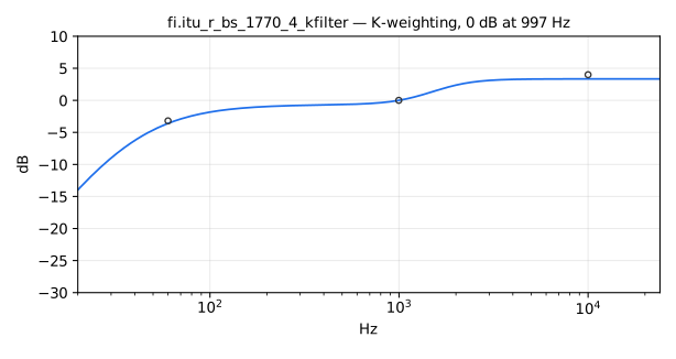
The prefilter from Recommendation ITU-R BS.1770-4 for loudness measurement. Also known as "K-filter". The recommendation defines biquad filter coefficients for a fixed sample rate of 48kHz (page 4-5). Here, we construct biquads for arbitrary samplerates. The resulting filter is normalized, such that the magnitude at 997Hz is unity gain 1.0.
Please note, the ITU-recommendation handles the normalization in
equation (2) by subtracting 0.691dB, which is not needed with
itu_r_bs_1770_4_kfilter.
One option for future improvement might be, to round those filter
coefficients, that are almost equal to one. Second, the maximum
magnitude difference at 48kHz between the ITU-defined filter and
itu_r_bs_1770_4_kfilter is 0.001dB, which obviously could be
less.
Usage
_ : itu_r_bs_1770_4_kfilter : _
Test
fi = library("filters.lib");
os = library("oscillators.lib");
src = os.tosc(440);
itu_r_bs_1770_4_kfilter_test = src : fi.itu_r_bs_1770_4_kfilter;
References
Averaging Functions
(fi.)avg_rect
Moving average.
Usage
_ : avg_rect(period) : _
Where:
period: averaging frame duration in seconds
Test
fi = library("filters.lib");
ba = library("basics.lib");
no = library("noises.lib");
ma = library("maths.lib");
avg_rect_test = no.noise : fi.avg_rect(0.01);
avg_rect_slider_test = no.noise : fi.avg_rect(hslider("period", 0.01, 0.001, 0.1, 0.001));
avg_rect_modulated_test = no.noise : fi.avg_rect(0.001 + 0.019*tri) with { P = int(ma.SR/10); tri = 1 - abs(2*ba.period(P)/P - 1) : max(0) : min(1); };
avg_rect_jump_test = no.noise : fi.avg_rect(0.001 + 0.019*sq) with { P = int(ma.SR/10); sq = ba.period(2*P) < P; };
(fi.)avg_tau
Averaging function based on a one-pole filter and the tau response time. Tau represents the effective length of the one-pole impulse response, that is, tau is the integral of the filter's impulse response. This response is slower to reach the final value but has less ripples in non-steady signals.
Usage
_ : avg_tau(period) : _
Where:
period: time, in seconds, for the system to decay by 1/e, or to reach 1-1/e of its final value.
Test
fi = library("filters.lib");
ba = library("basics.lib");
no = library("noises.lib");
ma = library("maths.lib");
avg_tau_test = no.noise : fi.avg_tau(0.01);
avg_tau_slider_test = no.noise : fi.avg_tau(hslider("period", 0.01, 0.001, 0.1, 0.001));
avg_tau_modulated_test = no.noise : fi.avg_tau(0.001 + 0.019*tri) with { P = int(ma.SR/10); tri = 1 - abs(2*ba.period(P)/P - 1); };
avg_tau_jump_test = no.noise : fi.avg_tau(0.001 + 0.019*sq) with { P = int(ma.SR/10); sq = ba.period(2*P) < P; };
References
(fi.)avg_t60
Averaging function based on a one-pole filter and the t60 response time.
This response is particularly useful when the system is required to
reach the final value after about period seconds.
Usage
_ : avg_t60(period) : _
Where:
period: time, in seconds, for the system to decay by 1/1000, or to reach 1-1/1000 of its final value.
Test
fi = library("filters.lib");
ba = library("basics.lib");
no = library("noises.lib");
ma = library("maths.lib");
avg_t60_test = no.noise : fi.avg_t60(0.01);
avg_t60_slider_test = no.noise : fi.avg_t60(hslider("period", 0.01, 0.001, 0.1, 0.001));
avg_t60_modulated_test = no.noise : fi.avg_t60(0.001 + 0.019*tri) with { P = int(ma.SR/10); tri = 1 - abs(2*ba.period(P)/P - 1); };
avg_t60_jump_test = no.noise : fi.avg_t60(0.001 + 0.019*sq) with { P = int(ma.SR/10); sq = ba.period(2*P) < P; };
References
(fi.)avg_t19
Averaging function based on a one-pole filter and the t19 response time.
This response is close to the moving-average algorithm as it roughly reaches
the final value after period seconds and shows about the same
oscillations for non-steady signals.
Usage
_ : avg_t19(period) : _
Where:
period: time, in seconds, for the system to decay by 1/e^2.2, or to reach 1-1/e^2.2 of its final value.
Test
fi = library("filters.lib");
ba = library("basics.lib");
no = library("noises.lib");
ma = library("maths.lib");
avg_t19_test = no.noise : fi.avg_t19(0.01);
avg_t19_slider_test = no.noise : fi.avg_t19(hslider("period", 0.01, 0.001, 0.1, 0.001));
avg_t19_modulated_test = no.noise : fi.avg_t19(0.001 + 0.019*tri) with { P = int(ma.SR/10); tri = 1 - abs(2*ba.period(P)/P - 1); };
avg_t19_jump_test = no.noise : fi.avg_t19(0.001 + 0.019*sq) with { P = int(ma.SR/10); sq = ba.period(2*P) < P; };
References
Zölzer, U. (2008). Digital audio signal processing (Vol. 9). New York: Wiley.
Kalman Filters
(fi.)kalman
The Kalman filter. It returns the state (a bus of size N).
Note that the only compile-time constant arguments are N and M.
Other arguments are capitalized because they're matrices, and it makes
reading them much easier.
Usage
kalman(N, M, B, R, H, Q, F, reset, u, z) : si.bus(N)
Where:
N: State size (constant int)M: Measurement size (constant int)B: Control input matrix (NxM)R: Measurement noise covariance matrix (MxM)H: Observation matrix (MxN)Q: Process noise covariance matrix (NxN)F: State transition matrix (NxN)reset: Reset trigger. Wheneverreset>0, the internal statexand covariance matrixPare reset.u: Control input (Mx1)z: Measurement signal (Mx1)
Example test programs
Demo 1 (N=1, M=1) (don't listen, just use oscilloscope):
process = fi.kalman(N, M, B, R, H, Q, F, reset, u, z) : it.interpolate_linear(filteredAmt, z)
with {
   B = 1.;
   R = 0.1;
   H = 1;
   Q = .01;
   F = la.identity(N);
   reset = button("reset");

   // Dimensions
   N = 1; // State size
   M = 1; // Measurement size

   freq = hslider("Freq", 1, 0.01, 10, .01);
   u = 0.; // constant input
   trueState = os.osc(freq)*.5 + u;
   noiseGain = hslider("Noise Gain", .1, 0, 1, .01);

   filteredAmt = hslider("Filter Amount", 1, 0, 1, .01) : si.smoo;

   measurementNoise = no.noise*noiseGain;
   z = trueState + measurementNoise; // Observed state
};
Demo 2 (N=2, M=1) (don't listen, just use oscilloscope)
process = fi.kalman(N, M, B, R, H, Q, F, reset, u, z)
with {
    B = par(i, N, 0);
    R = (0.1);
    H = (1, 0);
    Q = la.diag(2, par(i, N, .1));
    F = la.identity(N);
    reset = 0;
    u = si.bus(M);
    z = si.bus(M);

    // Dimensions
    N = 2; // State size
    M = 1; // Measurement size
};
Test
fi = library("filters.lib");
ba = library("basics.lib");
no = library("noises.lib");
ma = library("maths.lib");
kalman_test = fi.kalman(1, 1, 1, 0.1, 1, 0.01, 1, 0, 0, z) with { P = int(ma.SR/10); z = 0.5*(1 - abs(2*ba.period(P)/P - 1)) + 0.1*no.noise; };
References
Adaptive Filters
(fi.)lms, (fi.)nlms
Adaptive N-tap FIR filter trained by the (delayed-update) LMS rule:
the filter output y is the dot product of the adaptive weights with the
last N input samples, the error e = d - y is fed back, and each weight
moves along its instantaneous gradient: w_k <- w_k + mu * e * x@k.
nlms is the normalized variant: the step is divided by the energy of
the N input samples currently in the filter, making the convergence
rate independent of the input level (use it unless the input power is
known and constant).
The weight update uses the one-sample-delayed error (the standard "delayed LMS" that a causal sample loop imposes), which does not change the converged solution.
Usage
x, d : lms(N, mu) : _, _   // outputs: y (filter output), e (error)
x, d : nlms(N, mu) : _, _
Where:
N: number of adaptive weights (a constant numerical expression)mu: adaptation step; forlms, stability requiresmu < 2/(N*power(x)), while fornlmsvalues in (0, 2) are stable and 0.1-1.0 is typicalx: input signal (the reference fed to the adaptive FIR)d: desired signal
A converged identification of an unknown system H feeding
d = H(x) leaves the weights equal to the first N samples of the
impulse response of H, y equal to d, and e near zero.
Test
fi = library("filters.lib");
no = library("noises.lib");
lms_test = no.noise, (no.noise : @(3)*0.5 + no.noise@(1)*0.25) : fi.lms(8, 0.01);
nlms_test = no.noise, (no.noise : @(3)*0.5 + no.noise@(1)*0.25) : fi.nlms(8, 0.5);
References
- S. Haykin, "Adaptive Filter Theory", Prentice Hall.
- B. Widrow and S.D. Stearns, "Adaptive Signal Processing", Prentice Hall.
(fi.)adaptFIR
Generic adaptive N-tap FIR engine that lms and nlms are built on.
The filter output y is the dot product of the adaptive weights with the
last N input samples, the error e = d - y is the single feedback
signal, and each weight integrates its (one-sample-delayed) gradient
step: w_k <- w_k + step * e * x@k.
Unlike mu in lms, the step parameter is a signal, which makes
this the extension point for the whole family of adaptation rules:
nlms is adaptFIR with the step divided by the instantaneous input
energy, a leaky or gated LMS is adaptFIR with a step that decays or is
forced to 0 while adaptation should be frozen, a scheduled step
implements search-then-converge, and so on. Use lms/nlms directly
unless you need a custom rule.
Usage
x, d : adaptFIR(N, step) : _, _ // outputs: y (filter output), e (error)
Where:
N: number of adaptive weights (a constant numerical expression)step: adaptation step, as a signal evaluated at every sample; thelmsstability boundstep < 2/(N*power(x))applies to its instantaneous valuex: input signal (the reference fed to the adaptive FIR)d: desired signal
Example
// NLMS is one normalization away:
nlms(N, mu, x, d) = adaptFIR(N, mu / (ma.EPSILON + sum(k, N, x@k * x@k)), x, d);
// gated adaptation: freeze the weights below an input-level threshold
gatedLMS(N, mu, th, x, d) = adaptFIR(N, mu * (abs(x) > th), x, d);
Test
fi = library("filters.lib");
no = library("noises.lib");
adaptFIR_test = no.noise, (no.noise : @(3)*0.5 + no.noise@(1)*0.25)
    : fi.adaptFIR(8, 0.01);
References
- S. Haykin, "Adaptive Filter Theory", Prentice Hall.